Chapter 1
Describing data
As discussed in the opening lectures, an analytical and evidence-based approach to policymaking is a must for the modern & complex societies. As the famous engineer Edwards Deming put it, “Without data, you’re just another person with an opinion.” Data and its analysis are what distinguish well-designed policies from arbitrary and/or flawed ones. So, understanding the features & structure of data is an indispensable step of analysis.
A taxonomy of data types
Practically every sort of empirical analysis begins with a need to describe a data set & its various elements. So, we begin our journey to learn probability theory & statistics from this simple yet crucial task. Recall from the class discussion that data may come in two main forms: qualitative and quantitative. While qualitative data qualifies ‘things’, quantitative data quantifies ‘things’, as the terms suggest. In that, qualitative data often have a categorical nature. If the values of a categorical variable are orderable (sortable) then this categrorical variable is called an ‘ordinal’ categorical variable. Otherwise, it is a ‘nominal’ categorical variable. While the responses in a satisfaction survey are ordinal (consider 1: least liked to 5: most liked), indicators of gender are nominal (F: female and M: male). Note that it is not always trivial to come up with a judgment: while we can treat age categories of ‘young, middle-aged and old’ for people or class/year categories of ‘freshman, sophomore, junior and senior’ for students as ‘ordinal’, another researcher may choose to treat them as nominal. All we need to reveal is our capability to sort a categorical variable with a clear understanding stripped of value-judgments. For instance, one cannot simply put one of the genders on top of others, regardless of the underlying way of thinking.
Quantitative data is by definition numerical. It can be either discrete ‘as in the case of number of automobiles owned by households’ (one cannot own fractional automobiles) or continuous ‘as in the case of daily spending by households’. Household size, i.e., the number of people forming the household is discrete, number of cities in a country is discrete, etc. The case of people’s ages measured in years can be a little confusing: think about it.
Classifying data
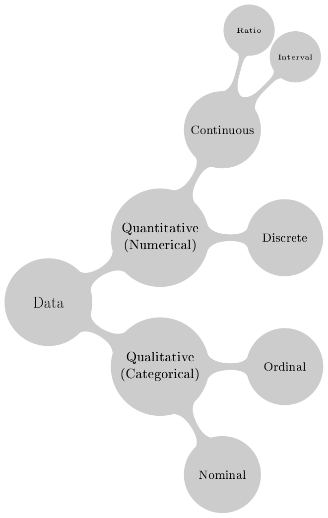
An important point regarding the continuous data is the distinction between ‘interval data’ and ‘ratio data’. A simple rule of thumb is: if there is an ‘absolute zero’ of the possible values of a data series, it is ‘ratio data’ & in the absence of an ‘absolute zero’ it is named ‘interval data’. A trivial example of this is the temperature measurements using the Kelvin (\(K\)) versus Celsius scale (\(^{\circ}C\)). While the Kelvin scale has an absolute zero, i.e. \(0 K\), the Celsius scale does not. Freezing point of pure water (under certain conditions) is \(0^{\circ}C\), yet this is not the lowest attainable temperature. Indeed, there are some \(273.15^{\circ}C\) more to go down until that point & \(-273.15^{\circ}C\) is defined as \(0 K\) and it is the lowest possible temperature in the Universe. While \(200 K\) is two times \(100 K\), \(200^{\circ}C\) is not two times \(100^{\circ}C\).
An easier example to understand the ratio data is the measurement of ‘mass’ (in kilograms, let’s say). Mass has an absolute zero, which is ‘\(0\) Kg’ & a \(20\) Kg object is two times as heavy as a \(10\) Kg object (assuming there is gravity).
What is a “data set”?
A data set is composed of one or more data items (series, variables) for use in analysis (in our case statistical analysis)
Each individual sub-item in a series is called a data value
There is often a clear correspondence between the data values of different data items involved, controlled by a primary key (observation number, date or a combination of both)
It is possible and often necessary to convert one data series ‘from numerical to categorical’. For instance, age data measured in ‘years lived’ can be expressed in terms of the qualifiers ‘young, middle-aged & old’. Note that, this transformation results in some loss of information. Clearly, a numerical age series tell more about the people surveyed compared to simple categorization. Still, when properly made, a good categorization of numerical values may prove very useful in statistical (or in econometric) analysis.
Frequency
In the Oxford English Dictionary, ‘frequency’ is defined as “the rate at which something occurs over a particular period of time or in a given sample”. Our understanding covers the cases of ‘being’ in addition to ‘occurring’ or happening: Frequency is the numerical measure of ‘how often something happens or how often some specific way of being is observed’. In that, as we can count car accidents in a certain hour, we can also count the people that survived a certain accident. So, we can count ‘things’ in time (we can call this temporal counting) and in space (we can call this spatial counting).
Frequency distribution
A frequency distribution is a tabular summary of how numerical values are distributed to classes in a data series.
First, determine the number of classes k, according to:
| Number of observations | \(k\) |
|---|---|
| <\(50\) | \(5-7\) |
| \(50-100\) | \(7-8\) |
| \(101-500\) | \(8-10\) |
| \(501-1,000\) | \(10-11\) |
| \(1,001-5,000\) | \(11-14\) |
| >\(5,000\) | \(14-20\) |
The table gives a rule of thumb and requires often your professional attention.
Second, determine the class width, \(w\):
\[w = \frac{Maximum - Minimum}{k}\] where \(Maximum\) is the ‘largest observation’ and \(Minimum\) is the ‘smallest observation’. Always round the formula result up, to find \(w\).
Third, construct the \(k\) classes; they are to be inclusive and non-overlapping.
Fourth, allocate your observations to classes and get the count of each class.
At the end, present your result as a table. What is obtained is a “frequency distribution table”.
Consider the age data of \(20\) people (\(20\) subjects) measured in years: \[\begin{array}{ccccc} 12 & 11 & 19 & 20 & 20 \\ 15 & 15 & 24 & 15 & 12 \\ 20 & 18 & 17 & 20 & 20 \\ 20 & 22 & 24 & 12 & 14 \end{array}\]
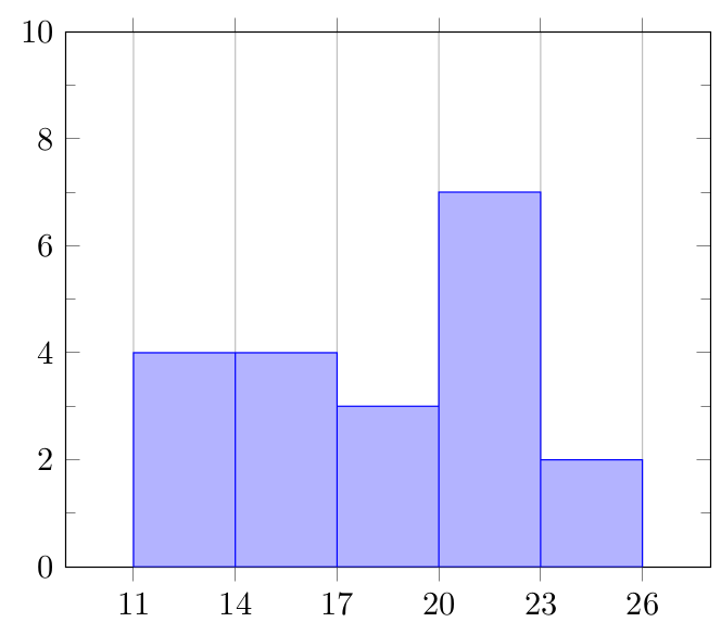
While summarizing the age data, it seems appropriate to use \(5\) classes following the rule of thumb given before. The \(max\) of our data series is \(24\) and the \(min\) is \(11\). Class width \(w\), then, is calculated as: \[w=\frac{24-11}{5}=2.6 \text{, always rounding up}\hat{\mid} w=3\] Having calculated the class width, beginning from the \(min\) value (\(11\) here) we establish our classes as \([11,14)\), \([14,17)\), \([17,20)\), \([20,23)\) and \([23,26]\). Pay attention to openness and closedness of classes (intervals) on the left and on the right.
Once the classes are ready, we carefully count the data values falling into each interval and prepare the following table, a table that we call the ‘frequency table’. \[\begin{array}{lc} Class & Frequency \\ {[11,14)} & 4 \\ {[14,17)} & 4 \\ {[17,20)} & 3 \\ {[20,23)} & 7 \\ {[23,26] } & 2 \end{array}\]
The final step is to prepare (draw) the histogram of our data.
Consider another researcher who prefers arbitrarily to use \(2\) classes. In this case, the class width (\(w\)) will be: \[w=\frac{24-11}{2}=6.5 \text{, always rounding up}\hat{\mid} w=7\] The classes will be \([11,18)\) and \([18,25)\), so our resulting frequency table will look like: \[\begin{array}{lc} Class & Frequency \\ {[11,18)} & 9 \\ {[18,25] } & 11 \end{array}\]
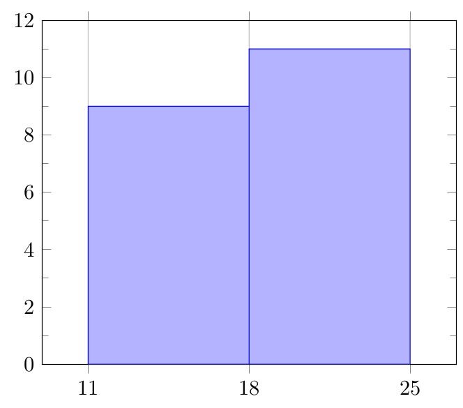
The final step is to prepare (draw) the histogram of our data again.
Which histogram (or frequency table) gives a better summary of the data? Avoid any confusions: the first histogram is the winner of the contest. It summarizes our data and conveys a tangible message. The second histogram, on the other hand, suffers from ‘oversummarizing’. Here take our discussion to its limits and consider a third researcher who prefers to use \(1\) class only. Why would that be nonsense?
What about categorical (qualitative) data? Consider the following data series which consists category markings for \(20\) people (\(20\) subjects), where \(Y\), \(M\) and \(O\) stand for ‘young’, ‘middle-aged’ and ‘old’, respectively.
\[\begin{array}{ccccc} Y & Y & O & M & Y \\ O & Y & O & O & Y \\ M & M & Y & M & O \\ O & M & Y & Y & M \end{array}\]
This time, forming a frequency table must be easier: we do not (indeed, we cannot) establish classes & simply count the frequency of each category:
\[\begin{array}{cc} Category & Frequency \\ {Y} & 8 \\ {M} & 6 \\ {O} & 6 \end{array}\]
The final step is to prepare (draw) the bar chart of our data. It is more than trivial; do it yourself.
Relative frequency distribution
Once the counts in a frequency distribution table are divided by the total number of observations & expressed as “percentages” or as ‘fractions between \(0\) and \(1\)’, the resulting table is called a “relative frequency distribution table”. By construction, relative frequencies of all classes add up to \(100\)% or \(1\).
Cumulative frequency distribution
Once the frequencies (counts) in a frequency distribution table are accumulated across classes, one row at a time and from the smallest to largest class, the resulting table is called a ‘cumulative frequency distribution table’.
Relative cumulative frequency distribution
Once the relative frequencies in a relative frequency distribution table are accumulated across classes, one row at a time and from the smallest to largest class, the resulting table is called a ‘relative cumulative frequency distribution table’.
In order to see the linkages between ‘frequency’, ‘relative frequency’, ‘cumulative frequency’ and ‘cumulative relative frequency’, examine the following table:
| Class | Frequency | Relative | Cumulative | Cumulative |
| frequency | frequency | relative | ||
| frequency | ||||
| \([10,17)\) | \(500\) | \(0.333\) | \(500\) | \(0.333\) |
| \([17,24)\) | \(250\) | \(0.167\) | \(750\) | \(0.500\) |
| \([24,31)\) | \(150\) | \(0.100\) | \(900\) | \(0.600\) |
| \([31,38]\) | \(600\) | \(0.400\) | \(\textbf{1500}\) | \(\textbf{1.000}\) |
| Total | \(\textbf{1500}\) | \(\textbf{1.000}\) | N.A. | N.A. |
Representation of distributions
Histogram and relative frequency polygon
A histogram is a graph that consists of vertical bars constructed on a horizontal line on which intervals are marked for the variable being displayed.
Horizontal intervals are the classes of a frequency or relative frequency distribution table
Height of each bar is the frequency or relative frequency associated
Warning: not the cumulative figures
Warning: consecutive bars for non-empty classes are to touch each other, i.e., no gaps
Histograms are traditionally used for continuous numerical data. When the midpoints of the top segment of each bar in a histogram are connected with line segments, what we obtain is called a frequency polygon. Note that a ‘bar chart’ resembles a histogram yet it differs in two main aspects: first, it is for categorical data & second, the bars in a bar chart are separated by a visible gap. Examples are provided in the upcoming exercises.
Symmetry and skewness
The shape of a distribution is said to be symmetric if the observations are balanced, or approximately evenly distributed, about its center. A distribution is skewed, or asymmetric, if the observations are not symmetrically distributed on either side of the center. A skewed-right distribution (sometimes called positively skewed) has a tail that extends farther to the right. A skewed-left distribution (sometimes called negatively skewed) has a tail that extends farther to the left.
O-give
An O-give, also called a cumulative line graph, is a line that connects points that are the cumulative percent of observations below the upper limit of each class (interval) in a cumulative frequency distribution. Even when not said so, an O-give is to present cumulative percentage figures. Beginning vertical value in an O-give is always \(0\) and ending vertical value is \(1\). Examples are provided in the upcoming exercises.
Exercise. Fill the empty cells in following table:
Interval Feq. Rel. freq.(%) Cum. freq. Rel. cum. freq.(%) \([0,20]\) \(20\) \(10\) \((20,40]\) \(80\) \((40,60]\) \(30\) \((60,80]\) \((80,100]\) \(20\) \(80\) \((100,120]\) Solution. The complete table is as follows:
Interval Freq. Rel. freq.(%) Cum. freq. Rel. cum. freq.(%) \([0,20]\) \(20\) \(10\) \(20\) \(10\) \((20,40]\) \(60\) \(30\) \(80\) \(40\) \((40,60]\) \(30\) \(15\) \(110\) \(55\) \((60,80]\) \(10\) \(5\) \(120\) \(60\) \((80,100]\) \(40\) \(20\) \(160\) \(80\) \((100,120]\) \(40\) \(20\) \(200\) \(100\) Consider the frequency histogram displayed below:
Draw the corresponding (relative frequency) o-give.
Solution. Prepare your Cartesian plane. The origin is \((0,0)\). Mark the following points on your graph space by paying attention to proportions: \((0,0)\), \((1.5,0.22)\), \((3.0,0.57)\), \((4.5,0.68)\), \((6.0,0.73)\), \((7.5,0.95)\), \((9.0,4.00)\). Then, connect these points with line segments from left to right. Once it is done, you will observe a properly drawn O-give. Make sure you have named the axes.
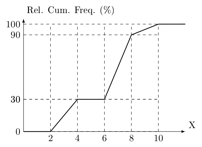
Consider the relative frequency o-give displayed below:
Draw the corresponding histogram. What can you say about the percentage of observations that takes a value less than or equal to \(6.5\) (if you need to estimate it what would be a reasonable estimate)? What can you say about the percentage of observations that takes a value greater than or equal to \(4.3\) (if you need to estimate it what would be a reasonable estimate)?
Solution.
Consider the classes of \([0,2]\), \((2,4]\), \((4,6]\), \((6,8]\) and \((8,10]\). Taking simple differences, reveal that relative frequencies of these classes are \(0\), \(0.3\), \(0\), \(0.6\) and \(0.1\). Locate these numbers on cartesian plane to obtain the histogram. Recall that for two successive classes which are non-empty, the bars must touch each other.
Relative frequency of \((6,8]\) is \(0.6\). \((6.5-6) /(8-6)=0.25\). So, approximately \(0.25 \times 0.6\), i.e., \(0.15\) is the frequency (relative) of \((6,6.5]\). Since the relative frequency of \([0,6]\) is \(0.3\), the frequency of \([0,6.5]\) becomes \(0.45\). If the given 0 -give has been drawn properly, then we expect our estimate to be reliable.
Use the same approach. The solution should yield \(0.70\).
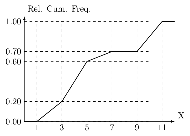
Consider the relative frequency o-give displayed below:
What can you say about the percentage of observations that takes a value between \(4.5\) and \(9.5\)?
Solution. Use the same approach. \(0.4/4+0.1+0+0.3/4\) yields \(0.275\).
A doctor’s office staff studied the waiting times for patients who arrive at the office with a request for emergency service. The following data with waiting times in minutes were collected over a one-month period:
\(2\), \(5\), \(10\), \(12\), \(4\), \(4\), \(5\), \(17\), \(11\), \(8\), \(9\), \(8\), \(12\), \(21\), \(6\), \(8\), \(7\), \(13\), \(18\), \(117\)
Construct a histogram for this data set by including all observations. Construct a histogram for this data set after excluding the value of \(117\). Note that you still have to show it on your histogram (but how?) Which histogram is more informative? Why?
Solution.
For ease in processing data sort/order the values as \(2\), \(4\), \(4\), \(5\), \(5\), \(6\), \(7\), \(8\), \(8\), \(8\), \(9\), \(10\), \(11\), \(12\), \(12\), \(13\), \(17\), \(18\), \(21\) and \(117\). The minimum is \(2\), the maximum is \(117\) and \(N\) is \(20\). \(5\) classes would work well here. Then, the class width becomes \((117-2) / 5=23\), rounding up always, \(24\). This means that our classes will be \([2,26]\), \((26,50]\), \((50,74]\), \((74,98]\) and \((98,122]\). When drawn (do it), this will turn out to be a funny histogram, as \(19\) observations will fall into the first class and only one observation (\(117\)) will fall into the last one.
When \(117\) is kept aside, the maximum becomes \(21\). Using \(5\) classes again, the class width becomes \((21-2) / 5\), which is \(3.8\), rounding up always, \(4\). Our classes will be \([2,6]\), \((6,10]\), \((10,14]\), \((14,18]\) and \((18,22]\). Respective frequencyies of these will be \(6\), \(6\), \(4\), \(2\) and \(1\). When drawn we will observe a neatly drawn histogram. (What about \(117\)?)
The second histogram is more informative. It gives us more details, like the shape of the distribution.
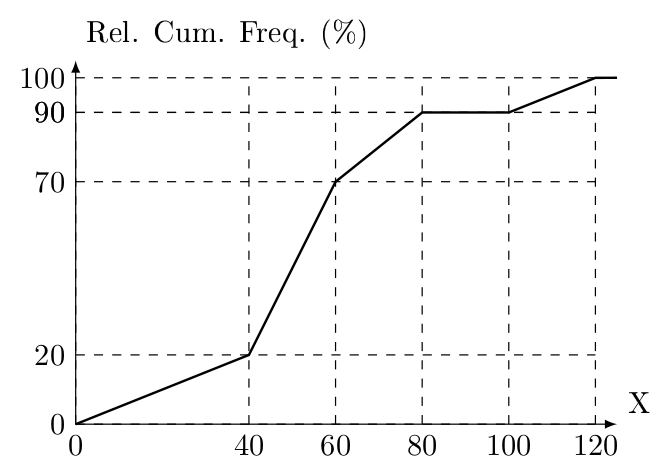
Consider the relative frequency o-give displayed below:
Based on the information above estimate the median and the 3rd quartile (\(Q_{3}\)).
Solution. Hint: For the median, find the horizontal value at which the O-give has the value of \(50\). For \(Q_{3}\), find the horizontal value at which the O-give has the value of \(75\).
In a data set, the frequency of the interval \((0,10]\) is \(0.10\), frequency of the interval \((10,20]\) is \(0.20\), frequency of the interval \((20,30]\) is \(0.30\) and frequency of the interval \((30,40]\) is \(0.40\). Construct the relative frequency O-give and calculate \(Q_{3}\) for this data set.
Solution. Solving this must be straightforward now. Do it and discuss with classmates.
Measures of central tendency
Measures of central tendency or measures of concentration indicate ‘where’ on the real number line our data series is. The three terms connotate:
Central tendency
Concentration
Location
As you’ll see in the upcoming classes, the knowledge of this is critically important to make several statistical assessments.
Measures of central tendency: Mode
The “mode”, whenever exists, is the most frequently occurring value in a data series.
If the series has one mode, it is called “unimodal”.
If the series has two modes, it is called “bimodal”.
If the series has three modes, it is called “trimodal”.
If the series has more than two modes, it may simply be called “multimodal”, use of the term “trimodal” is not that widespread in everyday professional use.
Note that, the mode is commonly used with (but not restricted to) categorical data.
Consider, \[X: 1, 2, 3, 3, 3, 4, 4, 5, 6, 7\] where \(N=10\). Among the values of \(X\), the most frequent (mostly repeated) value is \(3\), so we say \(Mode=3\). If X included another \(4\) like: \[X: 1, 2, 3, 3, 3, 4, 4, 4, 5, 6, 7\] where \(N=11\), then we would say the Modes are \(3\) and \(4\).
Measures of central tendency: Mean (Arithmetic mean)
For \(\left\{x_i\right\}_{i=1}^{N}\): \[\mu = \frac{\sum_{i = 1}^{N} x_{i}}{N}\] is called the “population mean”.
In addition, for \(\left\{x_i\right\}_{i=1}^{n}\): \[\bar{x} = \frac{\sum_{i = 1}^{n} x_{i}}{n}\] is called the ‘sample mean’
Considering, \[X: 1, 2, 3, 3, 3, 4, 4, 4, 5, 6, 7\] where \(N=11\), the mean is calculated as:
\[\begin{aligned} \mu & = \frac{\sum_{i = 1}^{N} x_{i}}{N} \\ & =\frac{1+2+3+3+3+4+4+4+5+6+7}{11} \\ & =3.81 \end{aligned}\]
In another case for \(X\), suppose the last value, i.e., \(7\), is replaced by \(42\); let’s call this data series as \(X'\): \[X: 1, 2, 3, 3, 3, 4, 4, 4, 5, 6, 42\] where \(N=11\) again, the mean becomes:
\[\begin{aligned} \mu & = \frac{\sum_{i = 1}^{N} x_{i}}{N} \\ & =\frac{1+2+3+3+3+4+4+4+5+6+42}{11} \\ & =7 \end{aligned}\]
As this example suggests, mean (\(\mu\)) is sensitive to outliers/extreme values. However, this sensitivity does not imply that \(\mu\) is a meaningless or a useless measure. On the contrary, it is a fundamental measure with many good statistical properties, as we will see in the upcoming chapters.
Consider,
| X | Frequency | Relative frequency |
|---|---|---|
| \([11,14)\) | \(4\) | \(4/20\) |
| \([14,17)\) | \(4\) | \(4/20\) |
| \([17,20)\) | \(3\) | \(3/20\) |
| \([20,23)\) | \(7\) | \(7/20\) |
| \([23,26]\) | \(2\) | \(2/20\) |
Using the midpoints and frequencies of classes:
\[\begin{aligned} \mu & =\frac{\frac{11+14}{2}\cdot4 + \frac{14+17}{2}\cdot4 + \frac{17+20}{2}\cdot3 + \frac{20+23}{2}\cdot7 + \frac{23+26}{2}\cdot2}{4+4+3+7+2} \\ & =18.35 \end{aligned}\]
is obtained.
Equivalently, one may use the relative frequencies of classes to calculate the same:
\[\begin{aligned} \mu & =\frac{11+14}{2}\cdot\frac{4}{20} + \frac{14+17}{2}\cdot\frac{4}{20} + \frac{17+20}{2}\cdot\frac{3}{20} + \frac{20+23}{2}\cdot\frac{7}{20} + \frac{23+26}{2}\cdot\frac{2}{20} \\ & =18.35 \end{aligned}\]
Measures of central tendency: Percentiles, Deciles and Quarties
The “p-th” percentile in a data series is the smallest value which is greater than \(p\)% of observations. If there are \(N\) observations, we find \[\frac{p}{100}(N+1)th\] ordered position and read the observation at this position as the \(p\)-th percentile.
The “\(d\)-th” decile in a data series is the smallest value which is greater than \(d\) tenths of observations. The “\(q\)-th” quartile in a data series is the smallest value which is greater than \(q\) quarters of observations.
While we imagine we are slicing our ordered data set into \(100\) while finding percentiles, we slice it into \(10\) while finding deciles, and we slice it into \(4\) while finding quartiles.
By definition \(P_{0} , Q_{0}, D_{0}\) are equal to the minimum observation and \(P_{100} , Q_{4}, D_{10}\) are equal to the maximum observation.
| 0th percentile | \(\rightarrow\) | 0th decile | \(\rightarrow\) | 0th quartile (\(Q_{0}\)) | \(\rightarrow\) | Minimum |
| 10th percentile | \(\rightarrow\) | 1st decile | ||||
| 20th percentile | \(\rightarrow\) | 2nd decile | ||||
| 25th percentile | \(\rightarrow\) | \(\rightarrow\) | \(\rightarrow\) | 1st quartile (\(Q_{1}\)) | ||
| 30th percentile | \(\rightarrow\) | 3rd decile | ||||
| 40th percentile | \(\rightarrow\) | 4th decile | ||||
| 50th percentile | \(\rightarrow\) | 5th decile | \(\rightarrow\) | 2nd quartile (\(Q_{2}\)) | \(\rightarrow\) | Median |
| 60th percentile | \(\rightarrow\) | 6th decile | ||||
| 70th percentile | \(\rightarrow\) | 7th decile | ||||
| 75th percentile | \(\rightarrow\) | \(\rightarrow\) | \(\rightarrow\) | 3rd quartile (\(Q_{3}\)) | ||
| 80th percentile | \(\rightarrow\) | 8th decile | ||||
| 90th percentile | \(\rightarrow\) | 9th decile | ||||
| 100th percentile | \(\rightarrow\) | 10th decile | \(\rightarrow\) | 4th quartile (\(Q_{4}\)) | \(\rightarrow\) | Maximum |
Measures of central tendency: Median
Among the many percentiles, “Median” has a special place. “Median” in a data series is the smallest value which is greater than \(50\)% of observations. It simply divides a data series into two equally-likely halves. Numerically, median is nothing but \(Q_{2}, P_{50}, D_{5}\), which are all the same.
Consider now a variable \(X\),
| 1st | 2nd | 3rd | 4th | 5th | 6th | 7th | 8th | 9th | 10th | 11th |
| \(1\) | \(1\) | \(2\) | \(3\) | \(5\) | \(8\) | \(13\) | \(21\) | \(34\) | \(55\) | \(89\) |
To find, for instance, the 30th percentile of \(X\) we calculate:
\[\begin{aligned} \frac{p}{100}(N+1)th & = \frac{30}{100}(11+1)th \\ & =3.6th \end{aligned}\]
Then, we find the observation value in the 3.6th position of the ordered data series. As seen here, there may not be such a physical position in data. As an approximation, we take the value of \(X\) in the 3rd position and add \(0.6\) times the difference between the value in 4th position and the value in 3rd position, i.e.,
\[\begin{aligned} P_{30} & =2+(3-2)\cdot0.6 \\ & =2.6 \end{aligned}\] is our 30th percentile.
To find the 80th percentile of \(X\) we calculate:
\[\begin{aligned} \frac{p}{100}(N+1)th & = \frac{80}{100}(11+1)th \\ & =9.6th \end{aligned}\]
\[\begin{aligned} P_{80} & =34+(55-34)\cdot0.6 \\ & =46.6 \end{aligned}\] So, \(46.6\) is our 80th percentile.
To find the Median, i.e., the 50th percentile of \(X\) we calculate:
\[\begin{aligned} \frac{p}{100}(N+1)th & = \frac{50}{100}(11+1)th \\ & =6th \end{aligned}\]
Without further calculations, \(8\) is our Median.
Consider another data series:
\[\begin{array}{ccccc} 2 & 3 & 4 & 6 & 7 \\ 8 & 9 & 9 & 10 & 10 \\ 11 & 11 & 11 & 11 & 13 \\ 14 & 18 & 19 & 19 & \textbf{19} \\ \textbf{21} & 21 & 22 & 22 & 23 \\ 23 & 23 & 24 & 24 & 24 \\ 24 & 25 & 25 & 25 & 26 \\ 26 & 26 & 26 & 26 & 49 \end{array}\]
Solve yourself to see that the Median is the 20.5th value of this data series and it is equal to \(20\).
Before moving forward, consider finally:
\[\begin{array}{ccccccccccc} Variable & 1st & 2nd & 3rd & 4th & \textbf{5th} & 6th & 7th & 8th & 9th & \textbf{Mean} \\ X & 1 & 3 & 6 & 10 & \textbf{15} & 21 & 28 & 36 & 1000 & \textbf{124.4} \\ X' & 1 & 3 & 6 & 10 & \textbf{15} & 21 & 28 & 36 & 45 & \textbf{18.3} \end{array}\]
Did you notice anything?
Where is my data? Five-number summary
When we give the five descriptive measures
\[minimum \leq Q_{1} \leq median \leq Q_{3} \leq maximum\] it is called a “five-number summary”. This is a somehow ancient and still useful tool to summarize data sets.
For a variable \(X\) given as: \[\begin{array}{ccccc}
2 & 3 & 4 & 6 & 7 \\
8 & 9 & 9 & 10 & 10 \\
11 & 11 & 11 & 11 & 13 \\
14 & 18 & 19 & 19 & \textbf{19} \\
\textbf{21} & 21 & 22 & 22 & 23 \\
23 & 23 & 24 & 24 & 24 \\
24 & 25 & 25 & 25 & 26 \\
26 & 26 & 26 & 26 & 49
\end{array}\] the five-number summary is \((2,10.25,20,24,49)\).
To make use of our knowledge gained up to this point, consider a data that is summarized with the following relative frequency o-give:
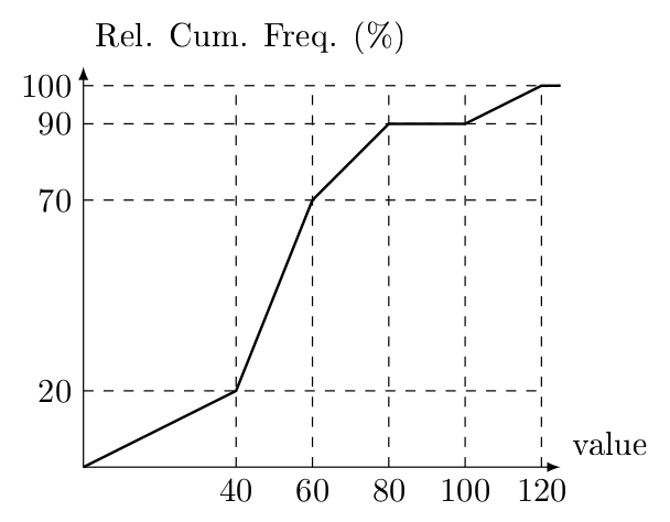
Based on the information above estimate the median, the mean, and the \(3\)rd quartile.
In order to reach a good solution, note that the median is the \(50\)th percentile and the 3rd quartile is the \(75\)th percentile. Under the assumption that data is uniformly distributed over each class interval, a relative cumulative frequency o-give gives information about the percentage of observations that takes a value less than or equal to a given number, we can use the o-give to estimate the median and the 3rd quartile using the o-give. On the graph we mark the points that correspond to \(50\)% and \(75\)%.
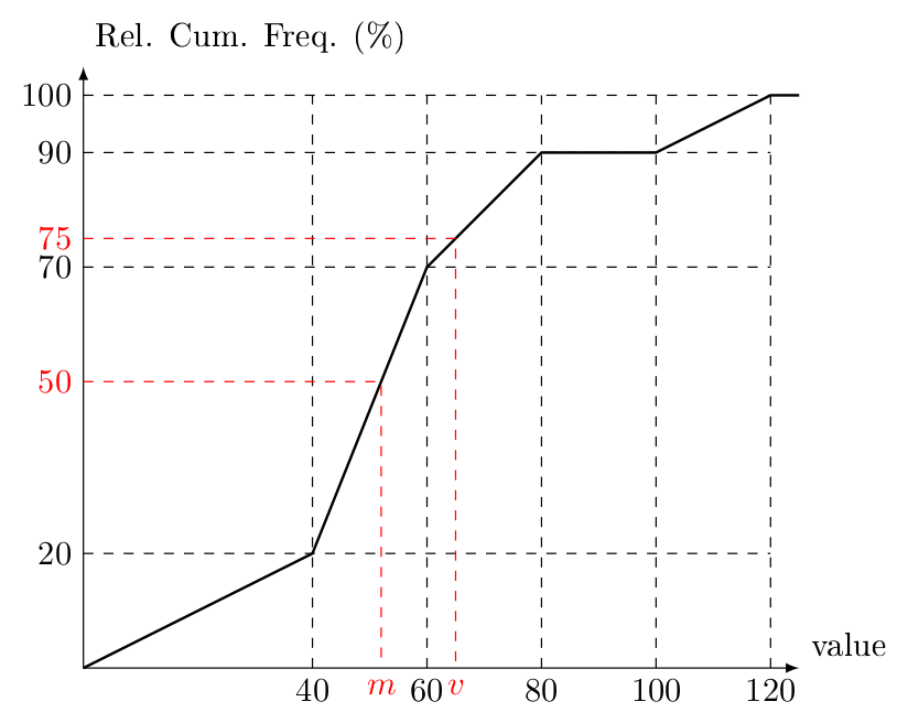
From similarity of triangles we have: \[\frac{m-40}{50-20} = \frac{60-40}{70-20}\]
which yields \[m = 40 + 30 \frac{20}{50} = 52\] Similarly \[\frac{v-60}{75-70} = \frac{80-60}{90-70}\] yields \[v = 60 + 5 \frac{20}{20} = 65\]
We will use \(CM_l\) to denote the class mark of the \(l\)th class interval (the center of the \(l\)th interval). We will use \(RF_l\) to denote the relative frequency of the observations that takes values in the \(l\)th class interval.
The assumption of data being uniformly distributed over each class interval that the following formula yields a “reasonable” estimate for the mean: \[RF_1 CM_1 + RF_2 CM_2 + RF_3 CM_3 + RF_4 CM_4 + RF_5 CM_5\] Thus our estimate for the mean is \[\begin{aligned} & (0.2-0) \frac{0+40}{2} + (0.7-0.2) \frac{40+60}{2} \\ & \qquad + (0.9-0.7) \frac{60+80}{2} + (0.9-0.9)\frac{80+100}{2} \\ & \qquad + (1.0-0.9) \frac{100+120}{2} \\ & = 54 \end{aligned}\]
Measures of dispersion
Measures of dispersion or measures of variation indicate how ‘spread’ on the real number line our data series is. The four terms connotate:
Dispersion
Variation
Spread
Fluctuation
Without properly assessing dispersion, the knowledge of location means only a little.
Measures of dispersion: Range
\[\operatorname{Range} = Largest obs - Smallest obs\] or \[\operatorname{Range} = Max - Min\] Range measures the length of the interval on the real number line spanned by our data set.
Measures of dispersion: Interquartile range
The interquartile range (IQR) is defined as: \[\operatorname{IQR} = Q_{3} - Q_{1}\] IQR measures the length of the interval on the real number line spanned by the “central \(50\)%” our data set.
Measures of dispersion: Box-Whisker plots
The five-number summary presented as a graph is called a Box-Whisker plot. Sometimes, near outliers and far outliers can also be added while constructing these plots.
Outliers
Near outliers
Far outliers
Measures of dispersion: Variance
For \(\left\{x_i\right\}_{i=1}^{N}\): \[\sigma^{2} = \frac{\sum_{i = 1}^{N} (x_{i} - \mu)^2}{N}\] is called the “population variance”, and for \(\left\{x_i\right\}_{i=1}^{n}\): \[s^{2} = \frac{\sum_{i = 1}^{n} (x_{i} - \bar{x})^2}{n-1}\] is called the ‘sample variance’
Consider: \[\begin{array}{ccccccc} 1 & 3 & 6 & 10 & 15 & 21 & 28 \end{array}\]
For this series, \(\mu=12\) (calculate yourself) and the variance is calculated as follows:
\[\begin{aligned} \sigma^{2} & = \frac{\sum_{i = 1}^{N} (x_{i} - \mu)^2}{N} \\ & =\frac{(1-12)^2+(3-12)^2+(6-12)^2+(10-12)^2+(15-12)^2+(21-12)^2+(28-12)^2}{7} \\ & =\frac{588}{7} \\ & =84 \\ \end{aligned}\]
A tabular approach may also be preferred:
| \(i\) | \(x_i\) | \(x_i-\mu\) | \((x_i-\mu)^2\) |
|---|---|---|---|
| 1 | 1 | -11 | 121 |
| 2 | 3 | -9 | 81 |
| 3 | 6 | -6 | 36 |
| 4 | 10 | -2 | 4 |
| 5 | 15 | 3 | 9 |
| 6 | 21 | 9 | 81 |
| 7 | 28 | 16 | 256 |
| 588 | |||
| \(\sigma^{2}=588/7=84\) |
Finally, one may calculate the sum of squares as \(1596\) and the mean as \(12\), and calculates the variance \(\sigma^2\) as \(1596/7-12^2\), which is \(84\).
Measures of dispersion: Standard deviation
For \(\left\{x_i\right\}_{i=1}^{N}\): \[\sigma = \sqrt{\sigma^{2}} = \sqrt{\frac{\sum_{i = 1}^{N} (x_{i} - \mu)^2}{N}}\] is called the “population standart deviation”, and for \(\left\{x_i\right\}_{i=1}^{n}\): \[s = \sqrt{s^{2}} = \sqrt{\frac{\sum_{i = 1}^{n} (x_{i} - \bar{x})^2}{n-1}}\] is called the ‘sample variance’
Consider the following data series:
\[\begin{array}{cccccc} 11 & 23 & 58 & 13 & 21 & 34 \\ 55 & 89 & 14 & 42 & 33 & 37 \\ 76 & 10 & 98 & 71 & 59 & 72 \\ 58 & 44 & 18 & 16 & 76 & 51 \\ 9 & 46 & 17 & 71 & 12 & 86 \\ 57 & 46 & 36 & 87 & 50 & 25 \\ 12 & 13 & 93 & 19 & 64 & 18 \\ 31 & 78 & 11 & 51 & 42 & 29 \end{array}\]
We are now asked to describe this data series, including its mean, five-number summary, range, interquartile range and variance. For ease in calculating the positional measures (quartiles here), it is a good practice to order the observations from the smallest to the largest, i.e., in ascending order:
\[\begin{array}{cccccc} 9 & 10 & 11 & 11 & 12 & 12 \\ 13 & 13 & 14 & 16 & 17 & 18 \\ 18 & 19 & 21 & 23 & 25 & 29 \\ 31 & 33 & 34 & 36 & 37 & 42 \\ 42 & 44 & 46 & 46 & 50 & 51 \\ 51 & 55 & 57 & 58 & 58 & 59 \\ 64 & 71 & 71 & 72 & 76 & 76 \\ 78 & 86 & 87 & 89 & 93 & 98 \end{array}\]
The following are then found:
\(N=48\)
\(Minimum=9\)
\(Maximum=98\)
\(\operatorname{Range}=Maximum-Minimum=98-9=89\)
\(\sum_{i = 1}^{N} x_{i}=2082\), so, \(\mu=2082/48=43.375\)
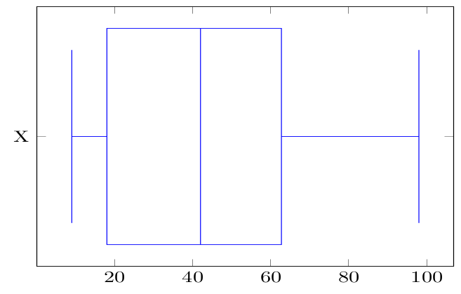
\(Q_2\) is at the \((48+1)\cdot0.5=24.5th\) position, \(Q_2=42\)
\(Q_1\) is at the \((48+1)\cdot0.25=12.25th\) position, \(Q_1=18\)
\(Q_3\) is at the \((48+1)\cdot0.75=36.75th\) position, \(Q_3=62.75\)
\((9,18,42,62.75,98)\) is the five-number summary
For the same data series (call it \(X\)), the Box-Whisker plot looks like:
Measures of dispersion: Coefficient of variation
Population coefficient of variation: \[\operatorname{CV} = \frac{\sigma}{\mu}100\% \text{ if } \mu \neq 0\] Sample coefficient of variation: \[\operatorname{CV} = \frac{s}{\bar{x}}100\% \text{ if } \bar{x} \neq 0\]
Measures of association for bivariate data
When we deal with one variable in our analysis, it is a case with “univariate” data. When we are concerned with patterns of change of two variables together, it is a case involving “bivariate” data. In these lecture notes,
\(\left\{x_i\right\}_{i=1}^{n_X}\) and \(\left\{x_i\right\}_{i=1}^{n_Y}\)
indicate univariate data, but
\(\left\{(x_i,y_i)\right\}_{i=1}^{n}\)
indicate bivariate data.
Notice that, bivariate data come in “pairs”, so one cannot change the correspondence between \(x\)’s and \(y\)’s.
Measures of association for bivariate data: Covariance
Covariance is a measure of the linear relationship between two variables. For \(\left\{(x_i,y_i)\right\}_{i=1}^{N}\), \[\operatorname{Cov}(x,y) = \sigma_{xy} = \frac{\sum_{i = 1}^{N} (x_i - \mu_{X})(y_i - \mu_{Y})}{N}\] For \(\left\{(x_i,y_i)\right\}_{i=1}^{n}\), \[\operatorname{Cov}(x,y) = s_{xy} = \frac{\sum_{i = 1}^{n} (x_i - \bar{x})(y_i - \bar{y})}{n}\]
Measures of association for bivariate data: Correlation
The correlation for \(\left\{(x_i,y_i)\right\}_{i=1}^{N}\) is given by \[\rho_{xy} = \frac{\sigma_{xy}}{\sigma_x \sigma_y}\] and for \(\left\{(x_i,y_i)\right\}_{i=1}^{n}\) \[r_{xy} = \frac{s_{xy}}{s_x s_y}\] When \(|r| \geq \frac{2}{\sqrt{n}}\) we say the (linear) relationship is strong enough (or significant). Notice that it is always the case that
\(-1 \leq \rho_{xy} \leq 1\)
\(-1 \leq r_{xy} \leq 1\)
Issues of unit and scale
Despite not paid enough attention by economists and business administration people, almost every data series comes with a unit and scale. For instance, if my income is \(TRY 96,000\), the unit is \(TRY\) (international code for Turkish lira) and the scale is not explicitly said. If we write it as \(TRY 96K\), the unit is again \(TR\) and the scale is “thousands”, so \(96\) means \(96,000\) here.
Consider \(\left\{(x_i,y_i)\right\}_{i=1}^{N}\) where \(x\) is the body weight in kilograms (kg) \(y\) is the height in centimeters (cm). Then,
| Measure | Unit |
|---|---|
| \(\mu_{x}\) | |
| \(\mu_{y}\) | cm |
| \(\sigma_{x}^2\) | \(kg^2\) |
| \(\sigma_{x}\) | kg |
| \(\sigma_{y}^2\) | \(cm^2\) |
| \(\sigma_{x}\) | cm |
| \(\operatorname{CV}_{x} = \frac{\sigma_{x}}{\mu{x}}\) | Unitless |
| \(\operatorname{CV}_{y} = \frac{\sigma{y}}{\mu{x}}\) | Unitless |
| \(\sigma_{xy}\) | \(kg.cm\) |
| \(\rho_{xy}\) | Unitless |
Similarly, quartiles, deciles and percentiles of a variable have the same unit as the variable. Range of a variable has the same unit as the variable. Interquartile range of a variable has the same unit as the variable. As a rule of thumb, linear operators do not alter the units.
Use of numerical scales is often a matter of practicality or convenience. Nobody likes to write \(123,000,000,000,000\) (except politicians) instead of writing \(123\) trillions or \(123.10^{12}\). One may need to learn two important practices of scaling numbers:
Logarithmic scales
Inverted scales
In this edition, these are left to readers as individual study.
Exercise. Consider a population with data values of:
\(5\), \(6\), \(3\), \(3\), \(6\), \(9\), \(10\), \(4\), \(10\), \(4\)Compute the mean, range, standard deviation, median, and \(Q_1\).
Solution. \(\mu=6\), \(\operatorname{Range} = \max - \min =7\), \(\sigma=2.61\), \(Q_{2}=5.5\) and \(Q_{1}=3.75\).
Find the mean, median, mode(s), variance, range, 1st quartile, and the 80th percentile of the data given below:
\(9\), \(13\), \(6\), \(7\), \(8\), \(6\), \(6\), \(9\), \(13\), \(13\)Solution. \(\mu=9\), \(Q_{2}=8.5\), modes are \(6\) and \(13\), \(\sigma^{2}=8\), \(\operatorname{Range}=7\), \(Q_{1}=6\) and \(P_{80}=13\).
A population has a range of R and it consists of two observations only. Calculate the variance of this data set.
Solution. \(x_{1}\) and \(x_{2}\) are the only two observations, and \(x_{2}-x_{1}=R\) is given (suppose \(x_{1}<x_{2}\). Then \(x_{2}-\mu=R / 2\) and \(x_{1}-\mu=-R / 2\). \[\begin{aligned} \sigma^{2} & =\frac{1}{2}\left[\left(x_{1}-\mu\right)^{2}+\left(x_{2}-\mu\right)^{2}\right] \\ & =\frac{1}{2}\left[(-R / 2)^{2}+(R / 2)^{2}\right] \\ & =\frac{1}{2} \cdot \frac{R^{2}}{2} \\ \sigma^{2} & =R^{2} / 4. \end{aligned}\]
A researcher argues that median equals the simple average of the first and third quartiles. By giving a numerical example, show that this is incorrect.
Solution. Find/make up your own example.
Let \(a\) and \(b\) be any given real numbers. Let \(x_1, x_2, \ldots, x_N\) and \(y_1, y_2, \ldots, y_N\) be two data sets such that, for any \(i=1, 2, \ldots, N\), and \(y_i=ax_i+b\).
What is the relation between the mean of the y-values and the mean of x-values? What is the relation between the variance of the y-values and the variance of x-values?
Solution. Needs some careful and patient elaboration.
\[\begin{aligned} \mu_{y} & =\frac{1}{N} \sum_{i=1}^{N} y_{i} \\ & =\frac{1}{N} \sum \left(a x_{i}+b\right) \\ & =\frac{1}{N} \sum a x_{i}+\frac{1}{N} \sum b \\ & =a \frac{1}{N} \sum x_{i}+\frac{1}{N} N b \\ & =a \mu_{x}+b \\ \mu_{y} & =a \mu_{x}+b \end{aligned}\]
\[\begin{aligned} \sigma_{y}^{2} & =\frac{1}{N} \sum_{i=1}^{N}\left(y_{i}-\mu_{y}\right)^{2} \\ & =\frac{1}{N} \sum\left(a x_{i}+b-a \mu_{x}-b\right)^{2} \\ & =\frac{1}{N} a^{2} \sum\left(x_{i}-\mu_{x}\right)^{2} \\ & =a^{2} \frac{1}{N} \sum\left(x_{i}-\mu_{x}\right)^{2} \\ & =a^{2} \sigma_{x}^{2} \\ \sigma_{y}^{2} & =a^{2} \sigma_{x}^{2} \end{aligned}\]
Consider a bivariate data consisting of the 1st midterm and 2nd midterm grades of \(216\) students. It is known that the 1st midterm grade of each student is \(8\)% less than his 2nd midterm grade. If the mean of the 2nd midterm grades is \(64\) and the variance is \(9\) what can you say about the correlation coefficient of this data?
Solution. Without any calculations we can say it is 1. Why?
If we remove a data point from a data series, variance decreases. True or false? Explain.
Solution. For a logical statement to be true, it must be true without any exceptions. Consider first \(\left\{1,5,9\right\}\) and second \(\left\{1,9\right\}\). Which set of values has a larger variance? What is your conclusion?
When we multiply each point in a data series by the same factor, the variance increases. True or false? Explain.
Solution. Consider \(y_{i}=k x_{i}, i=1,2, \ldots, N\). You have seen before that \[\sigma_{y}^{2}=k^{2} \sigma_{x}^{2}\] Then, \(\sigma_{y}^{2}\) is greater than \(\sigma_{x}^{2}\) only when \(k^{2}>1\), i.e., \(|k|>1\). So, the given statement is false (as we are able to find a counter example).
Below is the distribution of a variable \(X\) based on a sample of \(40\) observations. Compute the coefficient of variation.
X Frequency \(10-14\) \(8\) \(15-19\) \(16\) \(20-24\) \(u\) \(25-29\) \(4\) \(30-34\) \(2\) Solution. \(\mu=19\), \(\sigma^{2}=28.5\) and \(\sigma=5.34\). So, \[CV=\frac{\sigma}{\mu}=\frac{5.34}{19}=0.28\]
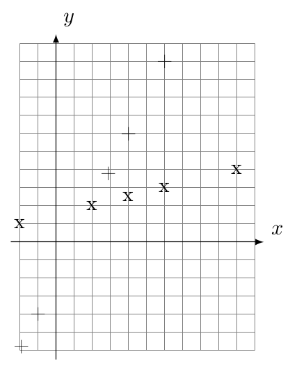
Consider the two populations of bivariate data:
Population 1 Population 2 \(x\) \(y\) \(x\) \(y\) \(2\) \(2\) \(2.9\) \(3.8\) \(6\) \(3\) \(-1\) \(-4\) \(10\) \(4\) \(-1.9\) \(-5.8\) \(4\) \(2.5\) \(4\) \(6\) \(-2\) \(1\) \(6\) \(10\) Find the covariance and correlation coefficient for each population. Plot the scatter plot for both populations. Standardize the \(x\) and \(y\) values in each population and plot the scatter plots for the standardized values.
Solution.
To find the covariance we first find the mean of \(x\) and \(y\) values for both populations: \[\begin{aligned} \mu_{1,x} & = \frac{1}{5} \left( 2 + 6 + 10 + 4 + (-2)\right) = 4 \\ \mu_{1,y} & = \frac{1}{5} \left( 2 +3 4 + 2.5 + 1\right) = 2.5 \\ \mu_{2,x} & = \frac{1}{5} \left( 2.9 + (-1) + (-1.9) + 4 + 6\right) = 2 \\ \mu_{2,y} & = \frac{1}{5} \left( 3.8 + (-4) + (-5.8) + 6 +10 \right) = 2 \end{aligned}\]
Thus \[\begin{aligned} \operatorname{Cov}_1 & = \frac{1}{5} \sum_{i=1}^5 (x_{1,i} - \mu_{1,x})(y_{1,i} - \mu_{1,y}) = 4 \\ \operatorname{Cov}_2 & = \frac{1}{5} \sum_{i=1}^5 (x_{2,i} - \mu_{2,x})(y_{2,i} - \mu_{2,y}) = 18.008 \approx 18 \\ \end{aligned}\] To find the correlation coefficient we first find the variances: \[\begin{aligned} \sigma_{1,x} & = \frac{1}{5} \sum_{i=1}^5 (x_{1,i} - \mu_{1,x})^2 = 16 \\ \sigma_{1,y} & = \frac{1}{5} \sum_{i=1}^5 (y_{1,i} - \mu_{1,y})^2 = 1 \\ \sigma_{2,x} & = \frac{1}{5} \sum_{i=1}^5 (x_{2,i} - \mu_{2,x})^2 = 9.006 \approx 9 \\ \sigma_{2,y} & = \frac{1}{5} \sum_{i=1}^5 (y_{2,i} - \mu_{2,y})^2 = 36.016 \approx 36 \\ \end{aligned}\] Thus \[\begin{aligned} \rho_1 & = \frac{\operatorname{Cov}_1}{\sigma_{1,x} \sigma_{1,y}} = \frac{4}{4 \cdot 1} = 1 \\ \rho_2 & = \frac{\operatorname{Cov}_2}{\sigma_{2,x} \sigma_{2,y}} = \frac{18}{3 \cdot 6} = 1 \\ \end{aligned}\]
Population \(1\) is represented with a “x” and population \(2\) with a “+” in the scatter plot below:
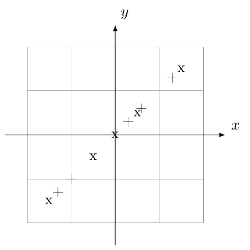
Standardized values are obtained by subtracting the corresponding mean from each value and dividing the result by the standard deviation:
Population 1 Population 2 \(x\) \(y\) \(x\) \(y\) \(-0.5\) \(-0.5\) \(0.3\) \(0.3\) \(0.5\) \(0.5\) \(-1\) \(-1\) \(1.5\) \(1.5\) \(-1.3\) \(-1.3\) \(0\) \(0\) \(0.6\) \(0.6\) \(-1.5\) \(-1.5\) \(1.3\) \(1.3\) The standardized values are plotted below:
Note that even though the original populations where on lines with different slope the standardized values are on a line with slope \(1\).
Chebyshev’s theorem (Chebyshev’s inequality)
For any data set with a mean of \(\mu\) and variance of \(\sigma^{2}\), and any \(k>1\), at least \[\left(1-\frac{1}{k^2}\right)100\%\] of the observations will take a value in the interval \([\mu-k\sigma,\mu+k\sigma]\).
Exercise. Consider a population with a mean of \(4\) and variance of \(36\). Using Chebyshev’s theorem find an interval that contains at least \(70\)% of the observations.
Solution. \(\mu=4\) and \(\sigma^{2}=36\), so \(\sigma=6\). \[\begin{gathered} \left(1-\frac{1}{k^{2}}\right) 100 \%=70 \% \\ 1-\frac{1}{k^{2}}=0.70 \\ \frac{1}{k^{2}}=0.30 \\ k^{2}=\frac{1}{0.30} \\ k=1.83. \end{gathered}\] So, the requested interval is: \[\begin{aligned} {[\mu-k \sigma, \mu+k \sigma] } & =[4-6(1.83), 4+6(1.83)] \\ & =[-6.95,14.95] \end{aligned}\]
The monthly charges for credit card holders at a department store have a mean of $\(250\) and a standard deviation of $\(100\). Use Chebyshev’s theorem to answer the following questions:
What can you say, for sure, about the percentage of card holders who will have monthly charges between $\(100\) and $\(400\)? Provide a range for the credit card charges that will include at least \(80\)% of all credit card customers.
Solution.
Use the same approach. For the interval \([100,400]\), \(k=1.5\). Reveal why. Then, this interval contains at least \[1-\frac{1}{1.5^{2}} \cdot 100 \%=(100-44) \%=56\%\] of all observations.
\([26.4,473.6]\) is the answer.
In a stock exchange average return over a year turns out to be \(1\)% with a standard deviation of \(2\)%. Over the same year, average exam grade in a university is \(60\) points with a standard deviation of \(24\) points. Which one has a higher variability, the returns or the grades?
Solution. \(CV\) for returns is \(2 \% / 1 \%=2\) and \(CV\) for grades is \(24 points/60 points =0.4\). So, returns have a higher variability.
When we replace a positive data value with its “additive inverse” in a data set, variance increases. Is this claim true or false? Either prove that it is true, or provide a counter example to show that it is false. Make sure you have used a formal mathematical notation.
Solution. Consider \(\left\{5,-7\right\}\) and \(\left\{-5,-7\right\}\). Which pair of values has higher variance? Then, come up with a conclusion.
Adding and multiplying terms over an index
If you’ve \(N\) numbers \(x_1, x_2, \ldots, x_N\), the sum of these numbers, \(S\), is: \[S = x_1 + x_2 + \cdots + x_N\] In expressing sums like this, we always write the first two terms, then three periods, then the last term. A shorter way to write S is: \[S = \sum_{i = 1}^{N} x_i\] where \(i\) is the index of \(x\), running from 1 to \(N\).
Unless otherwise specified, \(i\) increases by 1 every time, from 1 to \(N\). So, \(S = \sum_{i = 1}^{N} x_i\) is read as “sum of \(x_i\), \(i\) from 1 to \(N\)”. This means,
We’ll take \((i=1)\), \(x_1\) first,
take \((i=2)\): add \(x_2\),
take \((i=3)\): add \(x_3\)
\(\vdots\)
and taking the next \(x_i\) each time, we’ll take \((i=N)\) and add \(x_N\) the last.
For example, \[S = \Sigma_{i = 1}^{4} x_i = \sum_{i = 1}^{4} x_i = \sum_{i = 1}^{i = 4} x_i = x_1 + x_2 + x_3 + x_4\] If \(N\) is a number well-known in a problem: \[S = \sum x_i\] is a valid expression and it means “consider all \(x_i\)”,
Notice that \[\sum_{i = 1}^{N} = \left(\sum_{i = 1}^{N - 1}\right) + x_N = \left(\sum_{i = 1}^{N - 2}\right) + x_{N-1} + x_N\] and so forth.
In case we want to write \[x_1 + x_3 + \cdots + x_{2k-1}\] using our summation operator, we can write it as: \[\sum_{i = 1}^{k} x_{2i-1}\] As you’ve seen, wisely using i solves many problems.
Consider: \[S = 2\cdot x_1 + 2\cdot x_2 + \cdots + 2\cdot x_{N}\] which is equivalent to \[\sum_{i = 1}^{N} 2x_{i}\] \(S\), then, can be written as \[2\sum_{i = 1}^{N} x_{i}\] So, if each number in the sequence \(x_1, x_2, \ldots, x_N\) is multiplied by the same value which is not a function of \(i\), this value can be taken out of the summation sign \(\Sigma\).
Consider: \[S = x_1 + y_1 + x_2 + y_2 + \cdots + x_{N} + y_{N}\] Notice that, this is the same thing as: \[\sum_{i = 1}^{N} \left(x_{i} + y_{i}\right) = \sum_{i = 1}^{N} x_{i} + \sum_{i = 1}^{N} y_{i}\] Consider: \[S = \sum_{i = 1}^{N} x_{i} y_{i} = x_{1}y_1 + x_{2}y_{2} + \cdots + x_{N}y_{N}\] Notice that, \[S = \sum_{i = 1}^{N} x_{i} y_{i} \neq \left(\sum_{i = 1}^{N} x_{i}\right)\left(\sum_{i = 1}^{N} y_{i}\right)\] Sum of the products is not equal to product of the sums. Expand (write long) the expressions to see why not.
Consider: \[S = x_1 + 2x_2 + 3x_3 + \cdots + Nx_N\] How can we write this in short? \[S = \sum_{i = 1}^{N} ix_{i}\] Notice that: \[S = \sum_{i = 1}^{N} ix_{i} \neq \left(\sum_{i = 1}^{N} i\right)\left(\sum_{i = 1}^{N} x_{i}\right)\] Consider: \[S = \sum_{i = 1}^{N} \left(x_{i}\bar{y} + y_{i}\bar{x}\right)\] Since \(\bar{x}\) and \(\bar{y}\) are not indexed with \(i\), the expression is equal to: \[\bar{y} \sum_{i = 1}^{N} x_i + \bar{x} \sum_{i = 1}^{N} y_i\] Consider: \[\sum_{i = 1}^{N} x_{i}^2,\] Notice that \[\sum_{i = 1}^{N} x_{i}^2 \neq \left(\sum_{i = 1}^{N} x_i\right)^2\] Sum of the squares is not equal to square of the sum.
If you’ve \(N\) numbers \(x_1, x_2, \ldots, x_N\), the product of these numbers, \(P\), is: \[P = x_1 \cdot x_2 \cdots x_N\] In expressing products like this, we always write the first two terms, then three periods, then the last term. A shorter way to write \(P\) is: \[P = \prod_{i = 1}^{N} x_i\] where \(i\) is the index of \(x\), running from 1 to \(N\).
Consider: \[P = \prod_{i = 1}^{N} i\] What’s this?
It is nothing but \(P = \prod_{i=1}^{N} x_i\) with \(x_i=i\). So \(P\) equals: \[1\cdot 2\cdot 3\cdots N = N!\] Regarding our future purposes, an important property to remember is: \[ln\prod_{i = 1}^{N} x_i = \sum_{i = 1}^{N} ln x_i\] as we’ll use while writing Likelihood functions in ECON \(222\).
Finally, consider: \[\sum_{i = 0}^{N}\binom{N}{i} x^{N-i}y^{i}\] What’s this? Expand it to see:
\[= \binom{N}{0} x^{N-0}y^{0} + \binom{N}{1} x^{N-1}y^{1} + \cdots + \binom{N}{N} x^{N-N}y^{N}\] which is nothing but the binomial expansion
\((x+y)^N\)
as we’ll use while studying the Binomial and Poisson distributions in ECON \(221\).
Exercise.
Consider the expression for the population variance: \[\sigma^2 = \frac{1}{N}\sum_{i = 1}^{N}\left(x_i - \mu \right)^2\] and simplify it until you see: \[\sigma^2 = \frac{1}{N}\sum_{i = 1}^{N} x_{i}^2 - \mu^2\]
Solution. \[\begin{aligned} \sigma^{2} & =\frac{1}{N} \sum_{i=1}^{N}\left(x_{i}-\mu\right)^{2} \\ & =\frac{1}{N} \sum\left(x_{i}^{2}-2 \mu x_{i}+\mu^{2}\right) \\ & =\frac{1}{N} \sum x_{i}^{2}-\frac{2 \mu}{N} \sum x_{i}+\frac{1}{N} \sum \mu^{2} \\ & =\frac{1}{N} \sum x_{i}^{2}-2 \mu^{2}+\frac{1}{N} N \mu^{2} \\ \sigma^{2} & =\frac{1}{N} \sum x_{i}^{2}-\mu^{2}. \end{aligned}\] So, variance can be calculated by subtracting ‘the square of the mean of observations’ from ‘the mean of squared observations’.