Random variables

Earlier we entered the world of data and learned a rich collection of descriptive statistics, followed by developing a solid understanding of the probability theory. The knowledge of this chapter will now allow us to understand and practice the probability theory by means of the standard tools of calculus.

Formally, a random variable is a function from a sample space \(S\) to the set of real numbers \(\mathbb{R}\). Note at the very beginning that we denote random variables with uppercase letters and their particular values with the corresponding lowercase letters. So, a random variable \(X\) can take a value \(x\).

When we define the outcomes of a random experiment via a random variable, we can generalize the very structure of the experiment and get rid off our context-dependence.

After internalizing the knowledge of this chapter, we will be able to state and solve a long array of problems with more formalism. In the rest of this chapter, we will first study the concepts of ’Cumulative distribution function’ (\(CDF\)) and ’Probability distribution function’ (\(PDF\)). At the cost of a spoiler, we can say that \(CDF\) and \(PDF\) are the theoretical counterparts of O-give and histogram, respectively. Secondly, we will study the concepts of the Expected value and Variance along with their key properties. While doing so, we will create and refer to a number of ad hoc random variables. Ad hoc is a Latin phrase meaning literally ’to this’. In English, it is used to describe ’something that has been formed or used for a special and immediate purpose, without previous planning’. In that, until we reach the section entitled ’Random variablest and distributions: Discrete probability laws’, we will be creating, using and disposing several random variables that serve our specific scientific/ technical purposes.

On one hand, our discussion and use of those ad hoc random variables and distributions will prove quite useful to handle a long list of probabilistic or statistical cases/problems. On the other hand, staying ’ad hoc’ is not good for a full-fledged practice of science, as our journey will reveal. As a matter of fact, a rich set of probability laws (Discrete probability laws and Continuous probability laws) will allow us to categorize, model and solve a variety of real-world statistical problems in a sound as well as practical fashion. Note that the use of the term ’Law’ may not be the best alternative available in scientific nomenclature; yet, it is part of the tradition. Those who are not comfortable with the use of the term ’Law’ may replace it with the term ’Distribution’. As an example, ’Uniform probability, law’ and ’Uniform probability distribution’ are simply the same thing as each other.

Now, we can proceed with our quest to learn things. Recall our repeatedly used random expertment of ’tossing a fair coin’. Head and Tail (or, \(H\) and \(T\)) being the two sides of a coin, we already know the following:

\[\begin{aligned} & S=\left\{H, T\right\} \\ & \operatorname{P}\!\left(\text {Coin shows a Head}\right)=\operatorname{P}\!\left(H\right)=1 / 2 \\ & \operatorname{P}\!\left(\text {Coin shows a Tail}\right)=\operatorname{P}\!\left(T\right)=1 / 2 \end{aligned}\]

Upon these, we are allowed to define and study everything that is relevant. Despite its simplicity, such an approach lacks one important feature: mathematical generalization. Indeed, the real-world hosts a bunch of random experiments with two basic outcomes; a student to pass or to fail an exam, a patient to survive or not survive a sickness, an asteroid to hit or not to hit our planet Earth, and so on. Notice that each of these experiments look like tossing a coin. Furthermore, if the probability of passing the exam, the probability to survive and the probability to hit the Earth are equal to \(1/2\), these random experiments are ’identical’ with tossing a coin, except for the details of naming. So, why not to suggest a random variable \(X\) along with its probability distribution to address all these random experiments?

Consider \(X \in\left\{0,1\right\}\) (or \(x \in [0,1])\) for which \(\operatorname{P}\!\left(x=0\right)=1/2\) and \(\operatorname{P}\!\left(x=1\right)=1/2\). This is nothing but a direct equivalent of the random experiment of tossing a coin, without referring to coin explicitly. Let us leave this discussion for a while to consider another random experiment.

Now consider (or recall from our in-class discussions) the random experiment of drawing a number from the interval \([1,5]\) in a fully blind-folded fashion; so, there are infinitely many basic outcomes, which are the real numbers from \(1\) to \(5\) (as one cannot guarantee to pick intergers only, when blind-folded). With regard to this case, we already know the following:

\[S=\left\{x \mid x \in[1,5], x \in \mathbb{R}\right\}\]

or simply,

\[S=[1,5]\]

and

\[\operatorname{P}\!\left(\text{The number picked is } x\right)=0, \forall x\]

The final statement should trivially follow from chapter 4 (and should not sound weird to your ears anymore).

Following a similar agenda, to what we used in the case of tossing a fair coin above, we can say that the random experiment of picking a real number from \([1,5]\), from \([2,6]\), from \([3,7]\) or from \([1001,1005]\) should not differ. You may confirm this expectation once you have measured the length (size) of each of these intervals as \(4\) .

Define now \(Y \in[1,5]\) and leave this discussion aside until we cover the following definitions. Each of these definitions is crucial for our subsequent study of probability theory and statistics. Combining/pairing with your in-class notes, use these definitions to come up with a holistic picture of the things (objects) involved.

Cumulative distribution function: CDF

The cumulative distribution function or CDF of a random variable \(X\) is denoted by \(F_{X}\!\left(x\right)\) or \(F\!\left(x\right)\), and is defined as: \[F_{X}\!\left(x\right) = \operatorname{P}_{X}\!\left(X \leq x\right)\] or \[F\!\left(x\right) = \operatorname{P}\!\left(X \leq x\right)\]

Continuous and discrete random variables

A random variable \(X\) is continuous if \(F\!\left(x\right)\) is a continuous function of \(x\). A random variable \(X\) is discrete if \(F\!\left(x\right)\) is a step function of \(x\).

Additionally, the random variables \(X\) and \(Y\) are identically distributed if for every set \(A\), \[\operatorname{P}\!\left(X \in A\right) = \operatorname{P}\!\left(Y \in A\right)\] where this does not necessarily mean \(X = Y\). If \(X\) and \(Y\) are identically distributed, \[F_{X}\!\left(x\right) = F_{Y}\!\left(x\right), \forall x\]

Probability distribution functions

Probability distribution function: Case of discrete random variables

The probability distribution function PDF of a discrete random variable \(X\) is given by:

\[f_{X}\!\left(x\right) = \operatorname{P}\!\left(X = x\right), \forall x\] or \[f\!\left(x\right) = \operatorname{P}\!\left(X = x\right), \forall x\]

For discrete random variables, probability distribution function is also called the probability mass function.

Probability distribution function: Case of continuous random variables

The probability distribution function PDF of a continuous random variable \(X\) is the function \(f_{X}\!\left(x\right)\) that satisfies: \[F_{X}\!\left(x\right) = \int_{-\infty}^{x} f_{X}\!\left(t\right) dt, \forall x\] For continuous random variables, probability distribution function is also called the probability density function.

Connection between CDF and PDF

Using the Fundamental Theorem of Calculus, if \(f\!\left(x\right)\) is continuous \[\frac{d}{dx} F\!\left(x\right) = f\!\left(x\right)\] The analogy with the discrete case is almost exact. We “add up” the point probabilities \(f\!\left(x\right)\) to obtain interval probabilities \(F\!\left(x\right)\). With a slight abuse of the notation: \[\Delta F\!\left(x\right) = f\!\left(x\right)\]

Having been exposed to formal definitions of the functions and operators involved, now we will reconsider the random experiment of tossing a fair coin (discrete random variable case) and random experiment of picking a number from \([1,5]\) (continuous random variable case), in that order.

Using our newly acquired knowledge, we can now define the following:

\[\begin{aligned} & X \sim f\!\left(x\right) \\ & f\!\left(x\right)=\begin{cases} 1 / 2, & x=0 \\ 1 / 2, & x=1 \end{cases} \\ & F\!\left(x\right)=\begin{cases} 0, & x<0 \\ 1 / 2, & 0 \leq x<1 \\ 1, & x \leq 1 \end{cases} \end{aligned}\]

Here, \(X\) is nothing but the random variable that describes the outcomes of the random experiment of tossing a fair coin.

Consider also:

\[\begin{aligned} & Y \sim g(y) \\ & g(y)=\begin{cases} 1 / 4, & 1 \leq y \leq 5 \\ 0, & \text { otherwise } \end{cases} \\ & G(y)=\begin{cases} 0, & y<1 \\ \frac{y-1}{4}, & 1 \leq y \leq 5 \\ 1 & 5 \leq y \end{cases} \end{aligned}\]

You must have noticed that \(Y\) is the random variable that describes the outcomes of the random experiment of picking a number from \([1,5]\).

Since \(F\!\left(x\right)\) is a discrete function, \(X\) is a discrete random variable and since \(G(y)\) is a continuous function, \(Y\) is a continuous random variable.

In the cases of \(X \sim f\!\left(x\right)\) and \(Y \sim g(y)\) above, observe that:

\[\begin{aligned} & f\!\left(-0.5\right)=0 \\ & f\!\left(0.5\right)=0 \\ & f\!\left(1.5\right)=0 \\ & g(-0.5)=0 \\ & g(0)=0 \\ & g(1.5)=1 / 4 \\ & g(2.5)=1 / 4 \\ & g(5.1)=0 \\ & g(10)=0 \end{aligned}\]

Also, notice that:

\[\operatorname{P}\!\left(X=0\right)=f\!\left(0\right)=1 / 2\]

and

\[\operatorname{P}\!\left(Y=3\right)=0\]

while

\[g(3)=1 / 4\]

Your mind should be crystal clear in this distinction of probabilities and likelihoods for continuous random variables.

But, how we define/refer to probabilities and calculate them in the case of continuous random variables? The answer should be trivial to you: since the point probabilities are all zero for a continuous random variable, we can talk about the ’probabilities of intervals’ only. Then, the following calculation for the random variable \(Y\) above is legitimate:

\[\begin{aligned} \operatorname{P}\!\left(2 \leq Y \leq 4\right) & =\int_{2}^{4} g(y) d y \\ & =\int_{2}^{4} \frac{1}{4} d y \\ & =\left.\frac{y}{4}\right|_{2} ^{4} \\ & =\frac{4}{4}-\frac{2}{4} \\ & =\frac{2}{4} \\ & =\frac{1}{2} \end{aligned}\]

Alternatively,

\[\begin{aligned} \operatorname{P}\!\left(2 \leq Y \leq 4\right) & =G(4)-G(2) \\ & =\frac{4-1}{4}-\frac{2-1}{4} \\ & =\frac{3}{4}-\frac{1}{4} \\ & =\frac{2}{4} \\ & =\frac{1}{2} \end{aligned}\]

yields the same solution. Now, give an effort to show these solutions on the graphs of \(g(y)\) and \(G(y)\).

Expected Value

The expected value or mean of a random variable \(X\) is: \[\operatorname{E}\!\left(X\right) = \sum_{x} x f \left(x\right), \textit{if X is discrete}\] and \[\operatorname{E}\!\left(X\right) = \int_{-\infty}^{\infty} x f \left(x\right)dx, \textit{if X is continuous}\] provided that the sum or integral exists.

Variance and standard deviation

The variance of a random variable \(X\) is defined as: \[\operatorname{Var}\left(X\right) = \operatorname{E}\!\left(X - \ev{X}\right)^2\]

For a discrete random variable \(X\): \[\operatorname{Var}\left(X\right) = \sum_{x} \left(x - \operatorname{E}\!\left(X\right)\right)^2 f\!\left(x\right)\] where \[\operatorname{E}\!\left(X\right) = \sum_{x} x f \left(x\right)\] For a continuous random variable \(X\): \[\operatorname{Var}\left(X\right) = \int_{-\infty}^{\infty} \left(x - \operatorname{E}\!\left(X\right)\right)^2 f\!\left(x\right)dx\] where \[\operatorname{E}\!\left(X\right) = \int_{-\infty}^{\infty} x f \left(x\right) dx\]

The positive square root of \(\operatorname{Var}\left(X\right)\) is the standard deviation of \(X\). If \(X\) is a random variable with finite variance, then for any constants \(a\) and \(b\): \[\operatorname{Var}\left(aX+b\right) = a^2 \operatorname{Var}\left(X\right)\]

In a nutshell

An alternative and easier formula for the variance is given by: \[\operatorname{Var}\left(X\right) = \operatorname{E}\!\left(X^2\right) - \left(\operatorname{E}\!\left(X\right)\right)^2\] The simple proof is as follows: \[\begin{aligned} \operatorname{Var}\left(X\right) = \operatorname{E}\!\left(X - \ev{X}\right)^2 & = \operatorname{E}\!\left(X^2 - 2X\ev{X} + \left(\ev{X}^2\right)\right) \\ & = \operatorname{E}\!\left(X^2\right) - 2\operatorname{E}\!\left(X\ev{X}\right) + \operatorname{E}\!\left(\ev{X}\right)^2 \\ & = \operatorname{E}\!\left(X^2\right) - 2\operatorname{E}\!\left(X\right)\operatorname{E}\!\left(X\right) + \left(\operatorname{E}\!\left(X\right)\right)^2 \\ & = \operatorname{E}\!\left(X^2\right) - \left(\operatorname{E}\!\left(X\right)\right)^2 \end{aligned}\]

Regarding the same \(X\) and \(Y\) defined above, we can now study/compute the Expected value and the Variance:

\[\begin{aligned} & \operatorname{E}\!\left(X\right)=\sum_{x} x f\!\left(x\right) \\ & =0 \cdot \frac{1}{2}+1 \cdot \frac{1}{2} \\ & =\frac{1}{2} \end{aligned}\]

\[\begin{aligned} & \operatorname{Var}\left(X\right)=\sum_{x}(x-\operatorname{E}\!\left(X\right))^{2} f\!\left(x\right) \\ & =\left(0-\frac{1}{2}\right)^{2} \cdot \frac{1}{2}+\left(1-\frac{1}{2}\right)^{2} \cdot \frac{1}{2} \\ & =\frac{1}{4} \cdot \frac{1}{2}+\frac{1}{4} \cdot \frac{1}{2} \\ & =\frac{1}{4} \end{aligned}\]

\[\begin{aligned} & \operatorname{E}\!\left(X^{2}\right)=\sum_{x} x^{2} f\!\left(x\right) \\ & =0^{2} \cdot \frac{1}{2}+1^{2} \cdot \frac{1}{2} \\ & =\frac{1}{2} \end{aligned}\]

\[\begin{aligned} & \operatorname{Var}\left(X\right)=\operatorname{E}\!\left(X^{2}\right)-(\operatorname{E}\!\left(X\right))^{2} \\ & =\frac{1}{2}-\left(\frac{1}{2}\right)^{2} \\ & =\frac{1}{2}-\frac{1}{4} \\ & =\frac{1}{4} \end{aligned}\]

\[\begin{aligned} \operatorname{E}\!\left(Y\right) & =\int_{-\infty}^{\infty} y g(y) d y \\ & =\int_{1}^{5} y \frac{1}{4} d y \\ & =\left.\frac{y^{2}}{8}\right|^{5} \\ & =\frac{25}{8}-\frac{1}{8} \\ & =\frac{24}{8} \\ & =3 \end{aligned}\]

\[\begin{aligned} \operatorname{Var}\left(Y\right) & =\int_{-\infty}^{\infty}(y-\operatorname{E}\!\left(Y\right))^{2} g(y) d y \\ & =\int_{1}^{5}(y-3)^{2} \frac{1}{4} d y \\ & =\left.\frac{(y-3)^{3}}{12}\right|_{1} ^{5} \\ & =\frac{8}{12}-\left(-\frac{8}{12}\right) \\ & =\frac{16}{12} \\ & =\frac{4}{3} \end{aligned}\]

\[\begin{aligned} \operatorname{E}\!\left(Y^{2}\right) & =\int_{-\infty}^{\infty} y^{2} g(y) d y \\ & =\int_{1}^{5} y^{2} \frac{1}{4} d y \\ & =\left.\frac{y^{3}}{12}\right|_{1} ^{5} \\ & =\frac{125}{12}-\frac{1}{12} \\ & =\frac{124}{12} \\ = & \frac{31}{3} \end{aligned}\]

\[\begin{aligned} \operatorname{Var}\left(Y\right) & =\operatorname{E}\!\left(Y^{2}\right)-(\operatorname{E}\!\left(Y\right))^{2} \\ & =\frac{31}{3}-3^{2} \\ & =\frac{31-27}{3} \\ & =\frac{4}{3} \end{aligned}\]

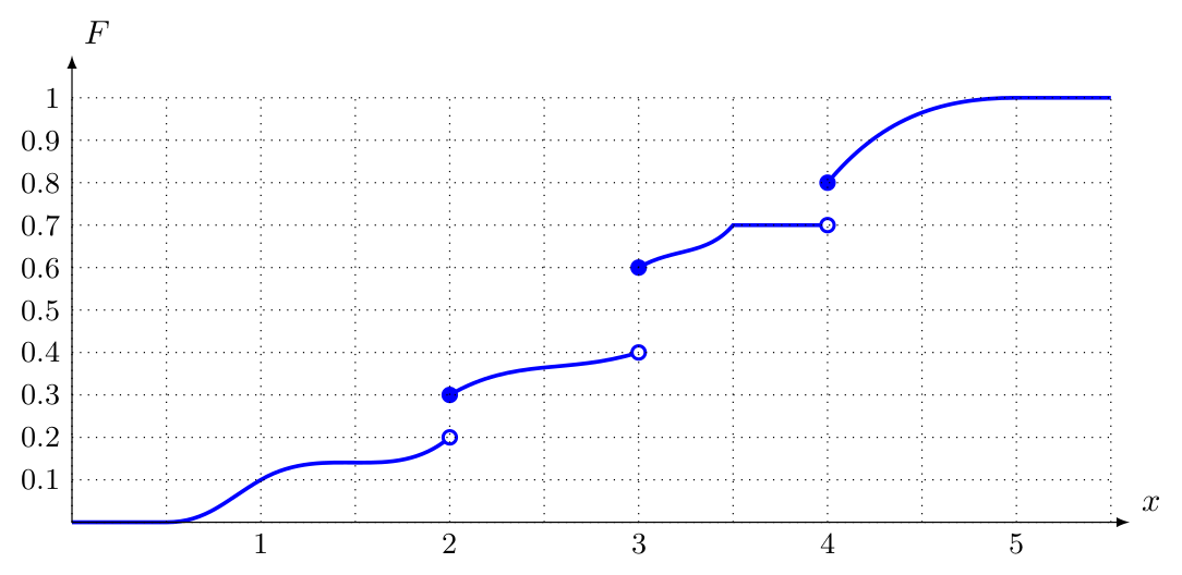
Exercise. Let \(X\) be a random variable with the following cumulative distribution function \(F\):

Calculate the following probabilities:

\(\operatorname{P}\!\left(X \leq 4\right)\) \(\operatorname{P}\!\left(2 < X \leq 4\right)\) \(\operatorname{P}\!\left(2 \leq X \leq 4\right)\) \(\operatorname{P}\!\left(3.5 \leq X < 4\right)\) \(\operatorname{P}\!\left(X = 4\right)\) \(\operatorname{P}\!\left(X > 3\right)\)

Solution.

\(\operatorname{P}\!\left(x \leq 4\right)=0.8\)

\(\operatorname{P}\!\left(2<x \leq 4\right)=0.5\)

\(\operatorname{P}\!\left(2 \leq x \leq 4\right)=0.6\)

\(\operatorname{P}\!\left(3.5 \leq x<4\right)=0\)

\(\operatorname{P}\!\left(x=4\right)=0.1\)

\(\operatorname{P}\!\left(x>3\right)=0.4\)

Let \(X\) be a discrete random variable with the following PDF, \(f\):

\(x\) \(1\) \(3\) \(5\) \(7\) \(9\)

\(f\!\left(x\right)\) \(0.4\) \(0.1\) \(0.2\) \(0.2\) \(0.1\)

\(\operatorname{P}\!\left(3 < X < 7\right)\) \(\operatorname{P}\!\left(3 < X < 7\,\middle|\,X > 5\right)\) Draw the graph of the CDF of \(X\). Find the expected value of \(X\).

Solution.

\(\operatorname{P}\!\left(3<x<7\right)=f\!\left(5\right)=0.2\)

\(\operatorname{P}\!\left(3<x<7\,\middle|\,x>5\right)=0\)

This exercise is left as self-study. \[\begin{aligned} \operatorname{E}\!\left(X\right)=\sum_{x} x f\!\left(x\right) & =1 \cdot 0.4+3 \cdot 0.1+5 \cdot 0.2+7.0 .2+9 \cdot 0.1 \\ & =0.4+0.3+1.0+1.4+0.9 \\ & =4 \end{aligned}\]

Explain why each of the following is or is not a valid probability distribution for a discrete random variable \(X\):

\(x\) \(0\) \(1\) \(2\) \(3\)

\(f\!\left(x\right)\) \(0.1\) \(0.3\) \(0.3\) \(0.2\)

\(x\) \(-2\) \(-1\) \(0\)

\(f\!\left(x\right)\) \(0.25\) \(0.50\) \(0.25\)

\(x\) \(4\) \(9\) \(20\)

\(f\!\left(x\right)\) \(-0.3\) \(0.4\) \(0.3\)

\(x\) \(2\) \(3\) \(5\) \(6\)

\(f\!\left(x\right)\) \(0.15\) \(0.15\) \(0.45\) \(0.35\)

Solution.

\(\sum_{x} f\!\left(x\right)=0.1+0.3+0.3+0.2\) \(=0.9<1.0\) (not valid).

\(f\!\left(x\right) \geq 0\) for all \(x\) values. \[\begin{aligned} \sum_{x} f\!\left(x\right) & =0.25+0.50+0.25 \\ & =1.0=1.0 \quad \text { (valid). } \end{aligned}\]

\(f\!\left(4\right)=-0.3<0 \quad\) (not valid).

\[\begin{aligned} & \sum_{x} f\!\left(x\right)=0.15+0.15+0.45+0.35>1 \\ & (\text { not valid). } \end{aligned}\]

The random variable \(X\) has the following discrete probability distribution:

\(x\) \(1\) \(3\) \(5\) \(7\) \(9\)

\(f\!\left(x\right)\) \(0.1\) \(0.2\) \(0.4\) \(0.2\) \(0.1\)

List the values \(x\) may assume. What value of \(x\) is the most probable? Graph the probability distribution. Find \(\operatorname{P}\!\left(X = 7\right)\) Find \(\operatorname{P}\!\left(X \geq 5\right)\) Find \(\operatorname{P}\!\left(X > 2\right)\) Find \(\operatorname{E}\!\left(X\right)\)

Solution.

\(x\) can take any of the values from \(\left\{1,3,5,7,9\right\}\).

\(f\!\left(5\right)\) is greater than all other \(f\!\left(x\right)\) valued; so, \(x=5\) is the most probable.

This exercise is left as self-study.

\(\operatorname{P}\!\left(x=7\right)=f\!\left(7\right)=0.2\)

\(\operatorname{P}\!\left(x \geq 5\right)=f\!\left(5\right)+f\!\left(7\right)+f\!\left(9\right)\) \(=0.4+0.2+0.1\) \(=0.7\)

\[\begin{aligned} \operatorname{P}\!\left(x>2\right) & =f\!\left(3\right)+f\!\left(5\right)+f\!\left(7\right)+f\!\left(9\right) \\ & =0.2+0.4+0.2+0.1 \\ & =0.9 \end{aligned}\]

\(\operatorname{E}\!\left(X\right)=\sum_{x} x f\!\left(x\right)=5\).

Consider the probability distributions,

\(x\) \(0\) \(1\) \(2\)

\(f\!\left(x\right)\) \(0.3\) \(0.4\) \(0.3\)

and

\(y\) \(0\) \(1\) \(2\)

\(f\!\left(y\right)\) \(0.1\) \(0.8\) \(0.1\)

Use your intuition to find the mean for each distribution. Which distribution appears to be more variable? Why?

Solution.

\(f\!\left(x\right)\) is symmetric around \(x=1\). \(f\!\left(y\right)\) is symmetric around \(y=1\). So, \(\operatorname{E}\!\left(X\right)=1\) and \(\operatorname{E}\!\left(Y\right)=1\).

\(X\) displays higher variation. Intuitively, "its values that are away from the expected value are more probable" compared to the case of \(Y\).

Every morning, my mother gives me a random amount of money according to the following PDF, where \(X\) is the random variable that measures the amount of money:

\(x\) \(20\) \(30\) \(40\) \(50\)

\(f\!\left(x\right)\) \(0.10\) \(0.20\) \(0.30\) \(0.40\)

Right after that, my sister takes out of my pocket a random amount of money according to the following CDF, where \(Y\) is the random variable that measures the amount of money:

\(y\) \(5\) \(10\) \(15\)

\(F\!\left(y\right)\) \(0.30\) \(0.70\) \(1.00\)

Then I leave home and spend all my money before the day ends. Create a random variable \(W\) which shows the net amount of money before I leave home in the morning. Calculate \(F\!\left(w\right)\) and present it in tabular format. Using these functions:

Calculate \(\operatorname{E}\!\left(X\right)\) Calculate \(\operatorname{E}\!\left(Y\right)\) Verify that \(\operatorname{E}\!\left(W\right)\) = \(\operatorname{E}\!\left(X\right) - \operatorname{E}\!\left(Y\right)\) Draw the graph of \(f\!\left(w\right)\) and mark the value of \(\operatorname{E}\!\left(W\right)\) on it Calculate \(\operatorname{Var}\left(W\right)\)

Solution. i. \[\begin{aligned} \operatorname{E}\!\left(x\right) & =\sum x f\!\left(x\right) \\ & =20 \cdot 0.10+30 \cdot 0.20+40 \cdot 0.30+50 \cdot 0.40 \\ & =2+6+12+20 \\ & =40 \end{aligned}\]

ii. First, we need to find \(g(y)\) :

\[\begin{aligned} & g(y)=\Delta G(y) \\ & g(5)=0.30 \leftarrow 0.30 \\ & g(10)=0.40 \leftarrow 0.70-0.30 \\ & g(15)=0.30 \leftarrow 1.00-0.70 \end{aligned}\]

\[\begin{aligned} \operatorname{E}\!\left(Y\right)=\sum y g(y) & =5 \cdot 0.30+10 \cdot 0.40+15 \cdot 0.30 \\ & =1.5+4+4.5 \\ & =10 \end{aligned}\]

iii. First, we need to find the PDF of \(W\), call it \(h(w)\). Find the possible values of \(W\) and calculate the probability for each \(w\). Those values are

\[\begin{aligned} & w \in\left\{5,10,15,20,25,30,35,40,45\right\} \\ & h(5)=f\!\left(20\right)g(15)=0.10 \cdot 0.30=0.03 \\ & h(10)=f\!\left(20\right)g(10)=0.10 \cdot 0.40=0.04 \\ & h(15)=f\!\left(20\right)g(5)+f\!\left(30\right)g(15)=0.10 \cdot 0.30+0.20 \cdot 0.30=0.09 \\ & h(20)=f\!\left(30\right)g(10)=0.20 \cdot 0.40=0.08 \\ & h(25)=f\!\left(30\right)g(5)+f\!\left(40\right)g(15)=0.20 \cdot 0.30+0.30 \cdot 0.30=0.15 \\ & h(30)=f\!\left(40\right)g(10)=0.30 \cdot 0.40=0.12 \\ & h(35)=f\!\left(40\right)g(5)+f\!\left(50\right)g(15)=0.30 \cdot 0.30+0.40 \cdot 0.30=0.21 \\ & h(40)=f\!\left(50\right)g(10)=0.40 \cdot 0.40=0.16 \\ & h(45)=f\!\left(50\right)g(5)=0.40 \cdot 0.30=0.12 \end{aligned}\]

Then,

\[\begin{aligned} \operatorname{E}\!\left(w\right)= & \sum w h(w) \\ = & 5 \cdot 0.03+10 \cdot 0.04+15 \cdot 0.09+20 \cdot 0.08 \\ & +25 \cdot 0.15+30 \cdot 0.12+35 \cdot 0.21+40 \cdot 0.16 \\ & +45 \cdot 0.12 \\ = & 0.15+0.4+1.35+1.6 \\ & +3.75+3.6+7.35+6.4 \\ & +5.4 \\ = & 30 \end{aligned}\]

From the previous parts we know that \(\operatorname{E}\!\left(X\right)=40\) and \(\operatorname{E}\!\left(Y\right)=10\). In this part, we found \(\operatorname{E}\!\left(W\right)=30\). So, \(\operatorname{E}\!\left(X\right)-\operatorname{E}\!\left(Y\right)=40-10=30=\operatorname{E}\!\left(W\right)\) \(\rightarrow\) verification done.

iv. Do on your own.

v. Calculate \(\operatorname{Var}\left(W\right)\) as:

\[\begin{aligned} \operatorname{Var}\left(W\right) & =\sum(w-\operatorname{E}\!\left(w\right))^{2} h(w) \\ & =(5-30)^{2} \cdot 0.03+(10-30)^{2} \cdot 0.04 \\ & +(15-30)^{2} \cdot 0.09+(20-30)^{2} \cdot 0.08 \\ & +(25-30)^{2} \cdot 0.15+(30-30)^{2} \cdot 0.12 \\ & +(35-30)^{2} \cdot 0.21+(40-30)^{2} \cdot 0.16 \\ & +(45-30)^{2} \cdot 0.12 \\ & =115 \end{aligned}\]

As an alternative:

\[\begin{aligned} \operatorname{E}\!\left(W^{2}\right)= & \sum w^{2} h(w) \\ & =25 \cdot 0.03+100 \cdot 0.04+225 \cdot 0.09 \\ & +400 \cdot 0.08+625 \cdot 0.15+900 \cdot 0.12 \\ & +1225 \cdot 0.21+1600 \cdot 0.16+2025 \cdot 0.12 \\ = & 1015 \end{aligned}\]

\[\begin{aligned} \operatorname{Var}\left(W\right) & =\operatorname{E}\!\left(W^{2}\right)-(\operatorname{E}\!\left(W\right))^{2} \\ & =1015-30^{2} \\ & =1015-900 \\ & =115 \end{aligned}\]

(As a follow-up exercise: calculate \(\operatorname{Var}\left(X\right)\) and \(\operatorname{Var}\left(Y\right)\) on your own, and verify that \(\operatorname{Var}\left(W\right)=\operatorname{Var}\left(X\right)+\operatorname{Var}\left(Y\right))\).

Consider \(X \sim f\!\left(x\right)=\frac{1}{4}, 4 \leq x \leq 8\), \(\quad Y \sim g(y)=\frac{1}{3}, 0 \leq y \leq 3\) and another random variable \(W\) which is defined as \(W=X-Y\). Calculate \(\operatorname{E}\!\left(X\right), \operatorname{E}\!\left(Y\right), \operatorname{E}\!\left(W\right)\), \(\operatorname{Var}\left(X\right), \operatorname{Var}\left(Y\right), \operatorname{Var}\left(W\right)\).

Solution.

\[\begin{aligned} \operatorname{E}\!\left(X\right)=\int_{-\infty}^{\infty} x f\!\left(x\right) d x=\int_{4}^{8} x \cdot \frac{1}{4} d x & =\left.\frac{1}{4} \frac{x^{2}}{2}\right|_{4} ^{8} \\ & =\frac{1}{8}(64-16) \\ & =6 \end{aligned}\]

\[\begin{aligned} \operatorname{E}\!\left(Y\right)=\int_{-\infty}^{\infty} y g(y) d y=\int_{0}^{3} y \frac{1}{3} d y & =\left.\frac{1}{3} \frac{y^{2}}{2}\right|_{0} ^{3} \\ & =\frac{1}{6}(9-0) \\ & =3 / 2 \\ \end{aligned}\]

\[\begin{aligned} \operatorname{E}\!\left(X^{2}\right)=\int_{-\infty}^{\infty} x^{2} f\!\left(x\right) d x=\int_{4}^{8} x^{2} \frac{1}{4} d x & =\left.\frac{1}{4} \frac{x^{3}}{3}\right|^{8} \\ & =\frac{1}{12}(512-64) \\ & =112 / 3 \end{aligned}\]

\[\begin{aligned} \operatorname{Var}\left(X\right) & =\operatorname{E}\!\left(X^{2}\right)-(\operatorname{E}\!\left(X\right))^{2} \\ & =\frac{112}{3}-36 \\ & =4 / 3 \end{aligned}\]

\[\begin{aligned} \operatorname{E}\!\left(Y^{2}\right)=\int_{-\infty}^{\infty} y^{2} g(y) d y=\int_{0}^{3} y^{2} \frac{1}{3} d y & =\left.\frac{1}{3} \frac{y^{3}}{3}\right|_{0} ^{3} \\ & =\frac{1}{9}(27-0) \\ & =3 \end{aligned}\]

\[\begin{aligned} \operatorname{Var}\left(Y\right) & =\operatorname{E}\!\left(Y^{2}\right)-(\operatorname{E}\!\left(Y\right))^{2} \\ & =3-\frac{9}{4} \\ & =3 / 4 \end{aligned}\]

Without finding \(h(w)\), the following can be written:

\[\begin{aligned} W=X-Y \rightarrow \operatorname{E}\!\left(W\right) & =\operatorname{E}\!\left(X\right)-\operatorname{E}\!\left(Y\right) \\ & =6-\frac{3}{2} \\ & =9 / 2 \\ \rightarrow \operatorname{Var}\left(W\right) & =\operatorname{Var}\left(X\right)+\operatorname{Var}\left(Y\right) \\ & =\frac{4}{3}-\frac{3}{4} \\ & =\frac{16-9}{12} \\ & =7 / 12 \end{aligned}\]

Another way to deal with \(W\) is:

\[\begin{aligned} & W \sim h(w), \quad h(w)=f\!\left(x\right) g(y) \\ & \operatorname{E}\!\left(W\right)=\int_{x=-\infty}^{\infty} \int_{y=-\infty}^{\infty}(x-y) f\!\left(x\right) g(y) d x d y \\ & =\int_{x=4}^{8} \int_{y=0}^{3}(x-y) \frac{1}{4} \frac{1}{3} d x d y \\ & =\left.\frac{1}{12} \int_{x=4}^{8} \frac{-(x-y)^{2}}{2}\right|_{y=0} ^{3} d x \\ & =-\frac{1}{24} \int_{4}^{8}\left[(x-3)^{2}-(x-0)^{2}\right] d x \\ & =-\frac{1}{24} \int_{4}^{8}(-6 x+9) d x \\ & =-\left.\frac{1}{24}\left(-6 \frac{x^{2}}{2}+9 x\right)\right|_{4} ^{8} \\ & =-\left.\frac{1}{24}\left(-3 x^{2}+9 x\right)\right|_{4} ^{8} \\ & =-\frac{1}{24}[(-3 \cdot 64+9 \cdot 8)-(-3 \cdot 16+9 \cdot 4)] \\ & =-\frac{1}{24}[-192+72+48-36] \\ & =-\frac{1}{24}(-108) \\ & =\frac{108}{24}=9 / 2 \text { (verifies } \operatorname{E}\!\left(W\right)=\operatorname{E}\!\left(X\right)-\operatorname{E}\!\left(Y\right) \text { ) } \end{aligned}\]

To calculate \(\operatorname{Var}\left(W\right)\) you do the following:

Calculate \(\operatorname{E}\!\left(W^{2}\right)\) \[\operatorname{E}\!\left(W^{2}\right)=\int_{x=4}^{8} \int_{y=0}^{3}(x-y)^{2} \frac{1}{4} \frac{1}{3} d x d y\]

Then, find \(\operatorname{Var}\left(W\right)\) \[\operatorname{Var}\left(W\right)=\operatorname{E}\!\left(W^{2}\right)-(\operatorname{E}\!\left(W\right))^{2}\]

If ’double integrals’ were not in the curriculum of MATH 105 or MATH 106 and if you do not have a prior knowledge of it, you may safely skip this last part.

\(x\)	\(1\)	\(3\)	\(5\)	\(7\)	\(9\)
\(f\!\left(x\right)\)	\(0.4\)	\(0.1\)	\(0.2\)	\(0.2\)	\(0.1\)

\(x\)	\(0\)	\(1\)	\(2\)	\(3\)
\(f\!\left(x\right)\)	\(0.1\)	\(0.3\)	\(0.3\)	\(0.2\)

\(x\)	\(-2\)	\(-1\)	\(0\)
\(f\!\left(x\right)\)	\(0.25\)	\(0.50\)	\(0.25\)

\(x\)	\(4\)	\(9\)	\(20\)
\(f\!\left(x\right)\)	\(-0.3\)	\(0.4\)	\(0.3\)

\(x\)	\(2\)	\(3\)	\(5\)	\(6\)
\(f\!\left(x\right)\)	\(0.15\)	\(0.15\)	\(0.45\)	\(0.35\)

\(x\)	\(1\)	\(3\)	\(5\)	\(7\)	\(9\)
\(f\!\left(x\right)\)	\(0.1\)	\(0.2\)	\(0.4\)	\(0.2\)	\(0.1\)

\(x\)	\(0\)	\(1\)	\(2\)
\(f\!\left(x\right)\)	\(0.3\)	\(0.4\)	\(0.3\)

\(y\)	\(0\)	\(1\)	\(2\)
\(f\!\left(y\right)\)	\(0.1\)	\(0.8\)	\(0.1\)

\(x\)	\(20\)	\(30\)	\(40\)	\(50\)
\(f\!\left(x\right)\)	\(0.10\)	\(0.20\)	\(0.30\)	\(0.40\)

\(y\)	\(5\)	\(10\)	\(15\)
\(F\!\left(y\right)\)	\(0.30\)	\(0.70\)	\(1.00\)

Random variables and distributions: Discrete probability laws

We consider here four (one being optional) discrete probability laws

Bernoulli distribution
Binomial distribution
Poisson distribution
Hypergeometric distribution
Geometric distribution
Negative Binomial distribution
Discrete Uniform distribution

Bernoulli distribution

Bernoulli distribution is also called Bernoulli trial or Bernoulli process. Consider an experiment consists of \(1\) trial and let there be two possible outcomes, success and fail.

Success \(\left(x = 1\right)\) with probability of \(P\)
Failure \(\left(x = 0\right)\) with probability of \(\left(1-P\right)\)

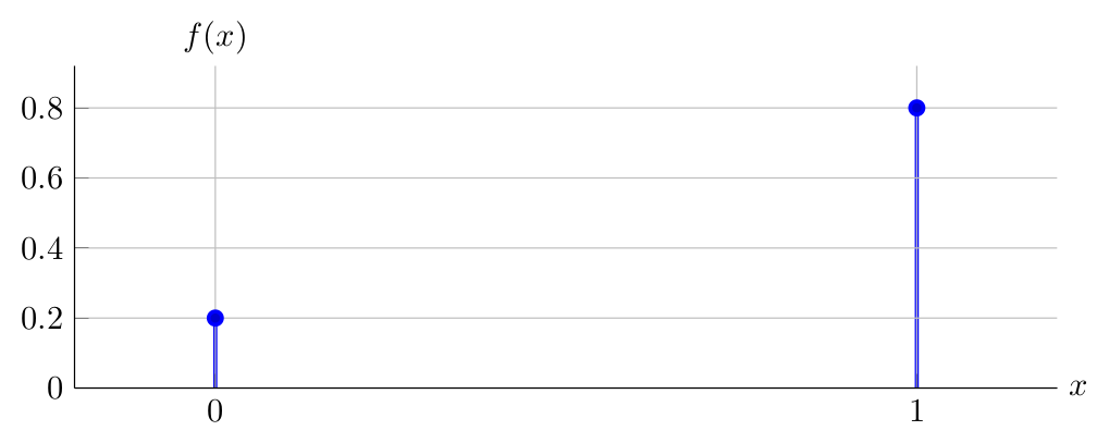
For \(X\sim \operatorname{Bernoulli}(P)\) \[\forall x \in \mathbb{R}, f\!\left(x\right) = \begin{cases} P & ,x = 1 \\ 1-P & ,x = 0 \\ 0 & ,otherwise \\ \end{cases}\]

Despite its simplicity, Bernoulli distributton is a stunningly useful one, as a building block of some other distributions.

Observe below the PDF of \(X \sim \operatorname{Bernoulli}(0.80)\):

Expected value and Variance:

\[\begin{aligned} \operatorname{E}\!\left(X\right)= \sum_{x=0}^{1} x f\!\left(x\right)= & 0 \cdot(1-P)+1 \cdot P \\ = & P \\ \end{aligned}\]

\[\begin{aligned} \operatorname{E}\!\left(X^2\right)= \sum_{x=0}^{1} x^{2} f\!\left(x\right)= & 0^{2}(1-P)+1^{2} \cdot P \\ = & P \\ \end{aligned}\]

\[\begin{aligned} \operatorname{Var}\left(X\right)= & \operatorname{E}\!\left(X^2\right)-(\operatorname{E}\!\left(X\right))^2 \\ = & P-P^{2} \\ = & \operatorname{P}\!\left(1-P\right) \end{aligned}\]

In a nutshell

A practical hint for deriving \(\operatorname{Var}\left(X\right)\)
As you have seen in the derivations of \(\operatorname{E}\!\left(X\right)\) and \(\operatorname{Var}\left(X\right)\) for the Bernoulli distribution, we first calculated the \(\operatorname{E}\!\left(X\right)\). This is an often seamless step. However, instead of attacking the \(\operatorname{Var}\left(X\right)\) directly, we preferred to calculate \(\operatorname{E}\!\left(X^{2}\right)\), which with the knowledge of \(\operatorname{E}\!\left(X\right)\) yields

\[\operatorname{Var}\left(X\right)=\operatorname{E}\!\left(X^{2}\right)-(\operatorname{E}\!\left(X\right))^{2}\]

In the remaining derivations of this chapter, notice the use of \[\operatorname{E}\!\left(X(X-1)\right)\] to facilitate easier derivation / calculation of \(\operatorname{Var}\left(X\right)\). Especially when the PDF of \(X\), ie., \(f\!\left(x\right)\) involves combinations, \(\operatorname{E}\!\left(X(X-1)\right)\) may be a life saver.

Notice that \(\operatorname{E}\!\left(X(X-1)\right)=\operatorname{E}\!\left(X^{2}-X\right)=\operatorname{E}\!\left(X^{2}\right)-\operatorname{E}\!\left(X\right)\)

So, \(\operatorname{E}\!\left(X^{2}\right)=\operatorname{E}\!\left(X(X-1)\right)+\operatorname{E}\!\left(X\right)\), and:

\[\begin{aligned} \operatorname{Var}\left(X\right) & =\operatorname{E}\!\left(X^{2}\right)-(\operatorname{E}\!\left(X\right))^{2} \\ & =\operatorname{E}\!\left(X(X-1)\right)+\operatorname{E}\!\left(X\right)-(\operatorname{E}\!\left(X\right))^{2} \end{aligned}\] Examine/ practice this hint along this chapter.

Binomial distribution

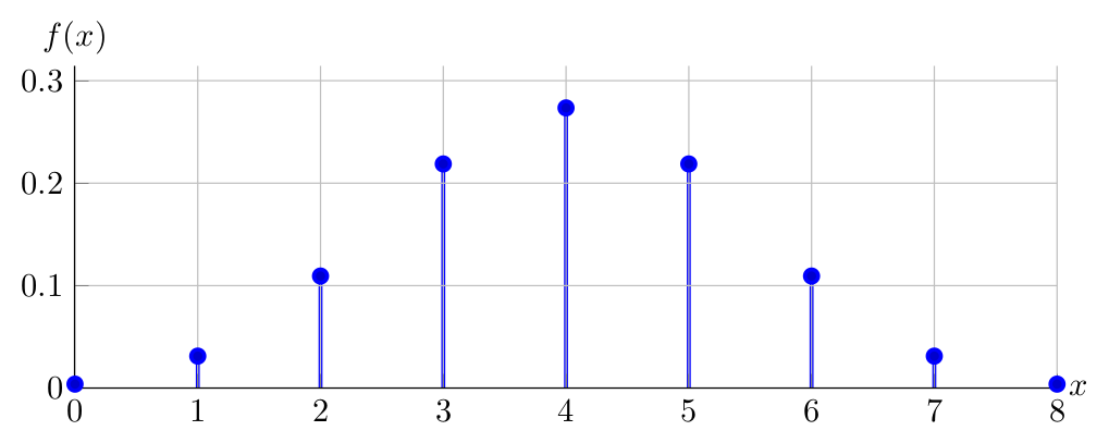
Consider an experiment which consists of \(n\) independent and identical Bernoulli trials;i.e, the probability of success \((P)\) is the same across all the trials and a trial’s outcome does not alter the outcomes of the subsequent trials. \(X\) being the number of successes in \(n\) trials, \(X\sim \operatorname{Binomial}(n, P)\), i.e., \(X\) has a Binomial distribution with parameters \(n\) and \(P\): \[\forall x \in \mathbb{R}, f\!\left(x\right) = \begin{cases} \binom{n}{x}P^{x}\left(1-P\right)^{n-x} & ,x = 0,1,2\ldots,n \\ 0 & ,otherwise \\ \end{cases}\]

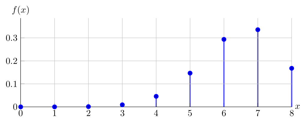
Observe below the PDF of \(X \sim \operatorname{Binomial}(8,0.80)\):

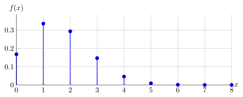
Then the PDF of \(X \sim \operatorname{Binomial}(8,0.20)\):

And finally the PDF of \(X \sim \operatorname{Binomial}(8,0.50)\):

Having compared the PDFs of \(\operatorname{Binomial}(8,0.80)\), \(\operatorname{Binomial}(8,0.20)\), \(\operatorname{Binomial}(8,0.50)\), can you identify the source of asymmetry of \(Binomial\) PDFs?

Expected value and Variance:

\[\begin{aligned} \operatorname{E}\!\left(X\right)= & \sum_{x=0}^{n} x \frac{n!}{x!(n-x)!}P^{x}(1-P)^{n-x} \\ = & nP\underbrace{\sum_{x=1}^{n}\frac{(n-1)!}{(x-1)!(n-x)!}P^{x-1}(1-P)^{n-x}}_{1} \\ = & nP \end{aligned}\]

\[\begin{aligned} \operatorname{E}\!\left(X^2\right)= & \sum_{x=0}^{n} x^{2} \frac{n !}{x!(n-x)!}P^{x}(1-P)^{n-x} \\ \end{aligned}\]

is not practical to work with. So, consider:

\[\begin{aligned} \operatorname{E}\!\left(X(X-1)\right)= & \sum_{x=0}^{n} x(x-1) \frac{n!}{x!(n-x)!}P^{x}(1-P)^{n-x} \\ = & n(n-1) P^{2} \underbrace{\sum_{x=2}^{n} \frac{(n-2)!}{(x-2)!(n-x)!}P^{x-2}(1-P)^{n-x}}_{1} \\ = & n(n-1)P^{2} \end{aligned}\]

This means: \[\begin{aligned} & \operatorname{E}\!\left(X^{2}\right)-\operatorname{E}\!\left(X\right)=n(n-1)P^{2} \\ & \operatorname{E}\!\left(X^{2}\right)=n(n-1) P^{2}+n P \\ \end{aligned}\]

Then,

\[\begin{aligned} \operatorname{Var}\left(X\right) & = \operatorname{E}\!\left(X^2\right)-(\operatorname{E}\!\left(X\right))^2 \\ & =n(n-1)P^{2}+nP-(nP)^{2} \\ & =n^{2}P^{2}-nP^{2}+nP-n^{2}P^{2} \\ & =nP-nP^{2} \\ & =nP(1-P) \end{aligned}\]

Poisson distribution

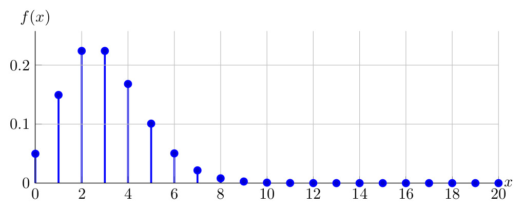
Consider an experiment which consists of counting the number of times a certain event occurs during a given unit of time or in a given area or volume. The probability that an event occurs in a given unit of time, area or volume is the same for all units. The number of events that occur in one unit of time, area or volume is independent of the number that occur in any other mutually exclusive unit. The mean (or expected, or typical) number of events in each unit is denoted by \(\lambda\). For \(X\sim \operatorname{Poisson}(\lambda)\): \[\forall x \in \mathbb{R}, f\!\left(x\right) = \begin{cases} \frac{\mathrm{e}^{-\lambda} \lambda^{x}}{x!} & ,x = 0,1,2\ldots \\ 0 & ,otherwise \\ \end{cases}\] Recall that, \(\mathrm{e}\) is called the Euler’s Number where \(\mathrm{e} = 2.71828\ldots\)

Observe below the PDF of \(X \sim \operatorname{Poisson}(3)\):

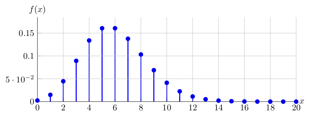
Then the PDF of \(X \sim \operatorname{Poisson}(6)\):

And finally the PDF of \(X \sim \operatorname{Poisson}(10)\):

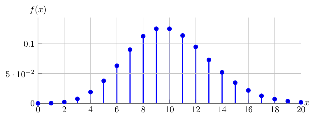
Is the last graph symmetric? Is it possible to have a \(\operatorname{Poisson}(\lambda)\) PDF which is symmetric? Why?

Expected Value and Variance:

\[\begin{aligned} \operatorname{E}\!\left(X\right)= & \sum_{x=0}^{\infty} x \frac{e^{-\lambda} \lambda^{x}}{x !} \\ = & e^{-\lambda} \sum_{x=0}^{\infty} x \frac{\lambda^{x}}{x !} \\ = & \lambda e^{-\lambda} \underbrace{\sum_{x=1}^{\infty} \frac{\lambda^{x-1}}{(x-1) !}}_{e^{\lambda}} \\ = & \lambda \\ \end{aligned}\]

\[\begin{aligned} \operatorname{E}\!\left(X^2\right)=\sum_{x=0}^{\infty} x^{2} \frac{e^{-\lambda}\lambda^{x}}{x!} \end{aligned}\]

is not useful againg. So, consider,

\[\begin{aligned} \operatorname{E}\!\left(X(X-1)\right)= & \sum_{x=0}^{\infty}x(x-1)\frac{e^{-\lambda}\lambda^{x}}{x!} \\ = & e^{-\lambda}\sum_{x=2}^{\infty}\frac{\lambda^{x}}{(x-2)!} \\ = & \lambda^{2} e^{-\lambda} \underbrace{\sum_{x=2}^{\infty}\frac{\lambda^{x-2}}{(x-2) !}}_{e^{\lambda}} \\ = & \lambda^{2} \\ \end{aligned}\]

This means,

\[\begin{aligned} \operatorname{E}\!\left(X^2\right)-\operatorname{E}\!\left(X\right)= & \lambda^2 \\ \operatorname{E}\!\left(X^2\right)= & \lambda^{2}+\lambda \\ \end{aligned}\]

Then,

\[\begin{aligned} \operatorname{Var}\left(X\right)= & \operatorname{E}\!\left(X^2\right)-(\operatorname{E}\!\left(X\right))^2 \\ = & \lambda^{2}+\lambda-\lambda^2 \\ = & \lambda \end{aligned}\]

How to derive Poisson distribution from Binomial distribution?

Consider a \(Binomial \left(n,p\right)\) process with: \[f\!\left(x\right) = \binom{n}{x} p^{x}\left(1-p\right)^{n-x}, x = 0,1,2, \ldots, n\] Define \[\lambda = np\] So, \[p = \frac{\lambda}{n}\] Re-writting \(f\!\left(x\right)\) as: \[f\!\left(x\right) = \lim_{n \to \infty} \binom{n}{x} \left(\frac{\lambda}{n}\right)^{x}\left(1-\frac{\lambda}{n}\right)^{n-x}\] the derivation yields. Now,

\[\begin{aligned} f\!\left(x\right) & = \lim_{n \to \infty} \binom{n}{x} \left(\frac{\lambda}{n}\right)^{x}\left(1-\frac{\lambda}{n}\right)^{n-x} \\ & = \left(\frac{\lambda^{x}}{x!}\right)\lim_{n \to \infty} \underbrace{\left[\frac{n!}{\left(n-x\right)!} \left(\frac{1}{n^{x}}\right)\right]}_{A}\underbrace{\left[\left(1 - \frac{\lambda}{n}\right)^{n}\right]}_{B}\underbrace{\left[\left(1 - \frac{\lambda}{n}\right)^{-x}\right]}_{C} \end{aligned}\] Consider now the parts \(A\), \(B\) and \(C\) separately:

The limit is \(1\); there are \(x\) terms linear in \(n\) in its numerator and \(x\) terms each of which is equal to \(n\) in its denominator
The limit is \(\mathrm{e}^{-\lambda}\); by definition of the Euler’s number.
The limit is \(1\) trivially.

Combining the limits: \[f\!\left(x|\lambda\right) = \operatorname{P}\!\left(X=x\,\middle|\,\lambda\right) = \frac{\lambda^{x} \mathrm{e}^{-\lambda}}{x!}\] is found.

The intuition is as follows: When we consider a Binomial process in which a success occurs with an infinitesimal probability in every infinitesimal time period and when there are infinitely many time periods as such, what yields for a finite time period is nothing but the Poisson distribution. The derivation can be carried out in reference to space rather than time, if you wish.

Hypergeometric distribution

Consider an experiment which consists of randomly drawing \(n\) elements without replacement from a set of \(N\) elements, \(r\) of which are successes and \(\left(N-r\right)\) of which are failures. \(X\) being the number of successes among \(n\) elements, \(X\sim Hypergeometric\left(N,r,n\right)\): \[\forall x \in \mathbb{R}, f\!\left(x\right) = \begin{cases} \frac{\binom{r}{x}\binom{N-r}{n-x}}{\binom{N}{n}} & ,x = \max \left\{0, n - \left(N-r\right)\right\}, \ldots, \min \left\{r,n\right\} \\ 0 & ,otherwise \\ \end{cases}\]

Expected Value and Variance:

\[\begin{aligned} \operatorname{E}\!\left(X\right)= & \sum_{x=0}^{n} x \frac{\left(\begin{array}{l} r \\ x \end{array}\right)\left(\begin{array}{c} N-r \\ n-x\end{array}\right)}{\left(\begin{array}{l} N \\ n\end{array}\right)} \\ = & \sum_{x=1}^{n} x \frac{\left(\begin{array}{c} r \\ x \end{array}\right)\left(\begin{array}{l} N-r \\ n-x\end{array}\right)}{\left(\begin{array}{l} N \\ n\end{array}\right)} \\ \end{aligned}\]

\[\begin{aligned} x\left(\begin{array}{l} r \\ x \end{array}\right)= & x\frac{r!}{x!(r-x)!} \\ = & r\frac{(r-1) !}{(x-1) !(r-x) !} \\ = & r\left(\begin{array}{l} r-1 \\ x-1 \end{array}\right) \\ \end{aligned}\]

\[\begin{aligned} \left(\begin{array}{l} N \\ n \end{array}\right)=\frac{N!}{n!(N-n)!}= & \frac{N(N-1)!}{n(n-1)!(N-n)!} \\ = & \frac{N}{n} \frac{(N-1) !}{(n-1) !(N-n) !} \\ = & \frac{N}{n}\left(\begin{array}{l} N-1 \\ n-1 \end{array}\right) \\ \end{aligned}\]

\[\begin{aligned} = & \sum_{x=1}^{n} \frac{r\left(\begin{array}{c} r-1 \\ x-1 \end{array}\right)\left(\begin{array}{c} N-r \\ n-x \end{array}\right)}{\frac{N}{n}\left(\begin{array}{c} N-1 \\ n-1 \end{array}\right)} \\ = & \frac{n r}{N} \underbrace{\sum_{x=1}^{n} \frac{\left(\begin{array}{c} r-1 \\ x-1\end{array}\right)\left(\begin{array}{c} N-r \\ n-x \end{array}\right)}{\left(\begin{array}{c} N-1 \\ n-1 \end{array}\right)}}_{1} \\ & =\frac{nr}{N} \end{aligned}\]

\[\begin{aligned} \operatorname{E}\!\left(X(X-1)\right) & =\sum_{x=0}^{n} x(x-1) \frac{\left(\begin{array}{c} r \\ x \end{array}\right)\left(\begin{array}{c} N-r \\ n-x \end{array}\right)}{\left(\begin{array}{l} N \\ n \end{array}\right)} \\ & =\sum_{x=2}^{n} x(x-1) \frac{\left(\begin{array}{c} r \\ x \end{array}\right)\left(\begin{array}{c} N-r \\ n-x \end{array}\right)} {\left(\begin{array}{l} N \\ n \end{array}\right)} \\ \end{aligned}\]

Notice that: \[\begin{aligned} x(x-1)\left(\begin{array}{c} r \\ x \end{array}\right) & =x(x-1) \frac{r !}{x !(r-x) !} \\ & =r(r-1) \frac{(r-2) !}{(x-2) !(r-x) !} \\ & =r(r-1)\left(\begin{array}{c} r-2 \\ x-2 \end{array}\right) \end{aligned}\]

and that:

\[\begin{aligned} \left(\begin{array}{c} N \\ n \end{array}\right)=\frac{N!}{n!(N-n)!} = & =\frac{N(N-1)(N-2)!}{n(n-1)(n-2)!(N-n)!} \\ = & \frac{N(N-1)}{n(n-1)}\left(\begin{array}{c} N-2 \\ n-2 \end{array}\right) \\ \end{aligned}\]

\[\begin{aligned} \operatorname{E}\!\left(X(X-1)\right)= & \sum_{x=2}^{n} \frac{r(r-1)\left(\begin{array}{c} r-2 \\ X-2 \end{array}\right)\left(\begin{array}{c} N-r \\ n-x \end{array}\right)}{\frac{N(N-1)}{n(n-1)}\left(\begin{array}{c} N-2 \\ n-2 \end{array}\right)} \\ = & \frac{nr}{N} \frac{(n-1)(r-1)}{N-1} \sum_{x=2}^{n} \frac{\left(\begin{array}{c} r-2 \\ X-2 \end{array}\right)\left(\begin{array}{c} N-r \\ n-x \end{array}\right)}{\left(\begin{array}{c} N-2 \\ n-2 \end{array}\right)} \end{aligned}\]

\[\begin{aligned} \operatorname{E}\!\left(X^2-X\right)= & \operatorname{E}\!\left(X^2\right)-\operatorname{E}\!\left(X\right) \\ = & \frac{n r}{N} \frac{(n-1)(r-1)}{N-1} \\ \operatorname{E}\!\left(X^2\right)= & \frac{n r}{N}\left(1+\frac{(n-1)(r-1)}{N-1}\right) \\ \end{aligned}\]

\[\begin{aligned} \operatorname{Var}\left(X\right)= & \operatorname{E}\!\left(X^2\right)-(\operatorname{E}\!\left(X\right))^2 \\ = & \frac{n r}{N}\left(1+\frac{(n-1)(r-1)}{N-1}\right)-\left(\frac{n r}{N}\right)^{2} \\ = & \frac{n r}{N}\left(1+\frac{(n-1)(r-1)}{N-1}-\frac{n r}{N}\right) \\ = & \frac{n r}{N}\left(\frac{N(N-1)+N(n-1)(r-1)-(N-1) n r}{N(N-1)}\right) \\ = & \frac{n r}{N} \cdot \frac{(N-n)(N-r)}{N(N-1)} \end{aligned}\]

Geometric distribution

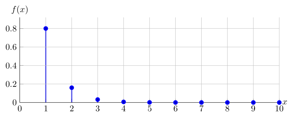
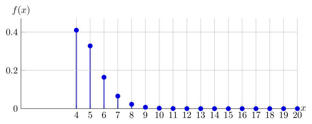
Consider an experiment which consists of a sequence of independent and identical Bernoulli trials; the expelriment ends when a (one) success is observed. \(X\) being the number of trials until one success, \(X \sim \operatorname{Geometric}(P)\), i.e., \(X\) has a geometric distribution with parameter \(P\): \[\forall x \in \mathbb{R}, f\!\left(x\right) = \begin{cases} (1-P)^{x-1}P & , x=1,2, \ldots \\ 0 & ,otherwise \\ \end{cases}\]

The construction of \(f\!\left(x\right)\) is intuitive as the experiment will yield \(x-1\) failures before the ’one and only’ success, which occurs at the end, by definition.

Observe below the PDF of \(X \sim Geometric(0.80)\):

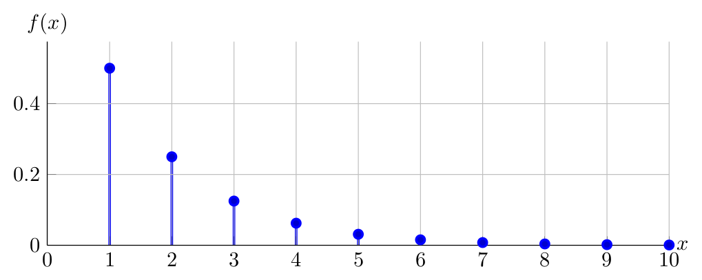
Observe below the PDF of \(X \sim Geometric(0.50)\):

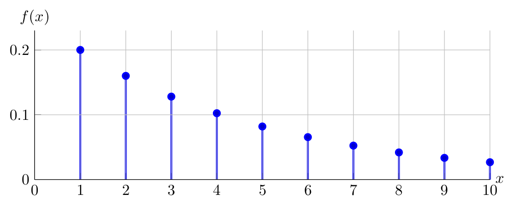
Observe below the PDF of \(X \sim Geometric(0.20)\) for \(1 \leq x \leq 10\)

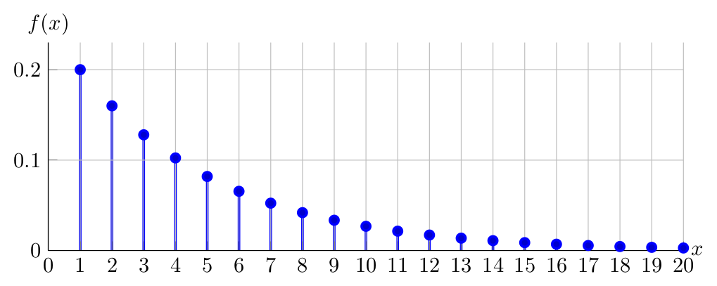
Observe below the PDF of \(X \sim Geometric(0.20)\) for \(1 \leq x \leq 20\)

Expected Value and Variance:

\[\begin{aligned} \operatorname{E}\!\left(X\right)= & \sum_{x=1}^{\infty} x(1-P)^{x-1} P \\ = & 1\operatorname{P}\!\left(1-P\right)^0+2\operatorname{P}\!\left(1-P\right)^1+3 \operatorname{P}\!\left(1-P\right)^{2}+\cdots \\ (1-P)\operatorname{E}\!\left(X\right)= & 1 \operatorname{P}\!\left(1-P\right)+2 \operatorname{P}\!\left(1-P\right)^{2}+3 \operatorname{P}\!\left(1-P\right)^{3}+\cdots \\ \operatorname{E}\!\left(X\right)-(1-P)\operatorname{E}\!\left(X\right)= & 1P+1\operatorname{P}\!\left(1-P\right)+1\operatorname{P}\!\left(1-P\right)^{2}+\cdots \\ \operatorname{E}\!\left(X\right)+(P-1)\operatorname{E}\!\left(X\right)= & P+\operatorname{P}\!\left(1-P\right)+\operatorname{P}\!\left(1-P\right)^{2}+\cdots \\ PE(X)= & \operatorname{P}\!\left(1+(1-P)+(1-P)^{2}+\cdots\right) \\ \operatorname{E}\!\left(X\right)= & \frac{1}{1-(1-P)}=\frac{1}{P} \end{aligned}\]

\[\begin{aligned} \operatorname{E}\!\left(X^2\right)= & \sum_{x=1}^{\infty}x^{2}(1-P)^{x-1}P \\ = & P\sum_{x=1}^{\infty}x^{2}(1-P)^{x-1} \\ = & P\frac{2-P}{P^{3}} \\ = & \frac{2-P}{P^{2}} \end{aligned}\]

Note that, denoting \(1-P=q\)

\[\begin{aligned} \sum_{x=1}^{\infty}x^{2} q^{x-1}=\frac{1+q}{(1-q)^{3}}= & \frac{1+1-P}{(1-1+P)^{3}} \\ = & \frac{2-P}{P^{3}} \end{aligned}\]

\[\begin{aligned} \operatorname{Var}\left(X\right)= & \operatorname{E}\!\left(X^2\right)-(\operatorname{E}\!\left(X\right))^2 \\ = & \frac{2-P}{P^{2}}-(\frac{1}{P})^{2} \\ = & \frac{1-P}{P^{2}} \\ \end{aligned}\]

Negative Binomial distribution

Consider an experiment which consists of a sequence of independent and identical Bernoulli trials; the expelriment ends when \(r\) successes are observed. \(X\) being the number of trials until \(r\) successes, \(X \sim \operatorname{Neg} \operatorname{Bin}(r,P)\), i.e., \(X\) has a Negative Binomial distribution with parameters \(r\) and \(P\):

\[\forall x \in \mathbb{R}, f\!\left(x\right) = \begin{cases} \binom{x-1}{r-1}P^{r}(1-P)^{x-r} & , x= r,r+1, \ldots \\ 0 & ,otherwise \\ \end{cases}\]

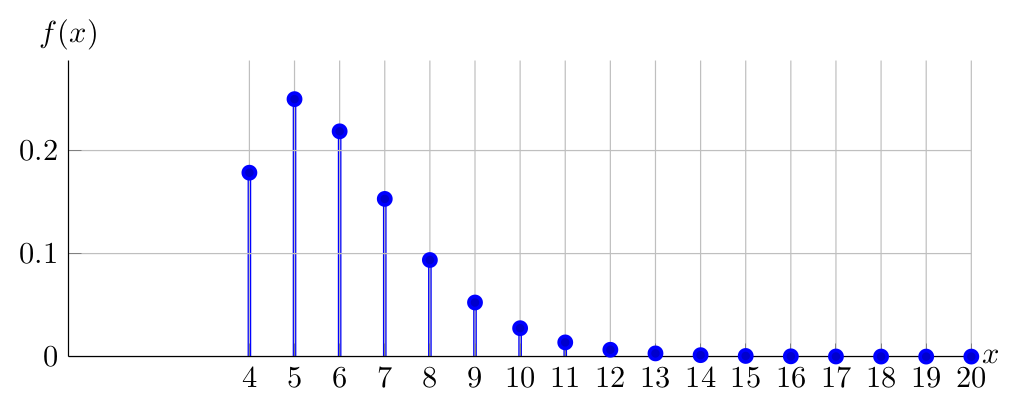
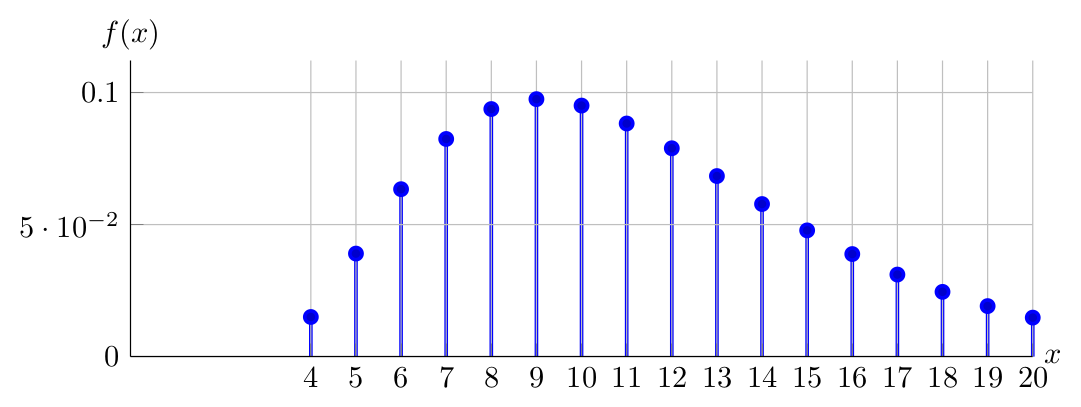
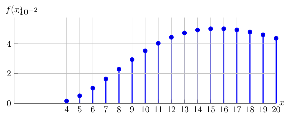
To develop an intuition of \(f\!\left(x\right)\), notice that the last Bernoulli trial yields success, with a probability of \(P\) and the \(x-1\) trials before that yield \(r-1\) successes with a probability of \(\binom{x-1}{r-1}P^{r-1}(1-P)^{x-r}\) according to a Binomial \((x-1,P)\) distribution, where the product of the two probabilities yield the Negative Binomial PDF. Observe below the PDF of \(X \sim NegativeBinomial(4,0.80)\):

Observe below the PDF of \(X \sim NegativeBinomial(4,0.65)\):

Observe below the PDF of \(X \sim NegativeBinomial(4,0.50)\):

Observe below the PDF of \(X \sim NegativeBinomial(4,0.35)\):

Observe below the PDF of \(X \sim NegativeBinomial(4,0.20)\):

Discrete Uniform distribution

\[\begin{aligned} & X \sim \text { Uniform }(a, b), a \leq x \leq b \in Z \\ & n=b-a+1 \\ & f\!\left(x\right)=\frac{1}{n} \\ & \operatorname{E}\!\left(X\right)=\frac{a+b}{2} \\ & \operatorname{Var}\left(X\right)=\frac{n^{2}-1}{12} \end{aligned}\]

\(X \sim \operatorname{Uniform}(a, b)\)

Expected Value and Variance:

\[\begin{aligned} n= & b-a+1 \\ f\!\left(x\right)= & \frac{1}{n} \\ \end{aligned}\]

\[\begin{aligned} \operatorname{E}\!\left(X\right) = & \sum_{x=a}^{b} x\frac{1}{n} \\ = & \frac{na+\frac{(b-a)(b-a+1)}{2}}{n} \\ = & \frac{2na+(b-a)n}{2n} \\ = & \frac{2a+b-a}{2} \\ = & \frac{a+b}{2} \end{aligned}\]

\[\begin{aligned} \operatorname{E}\!\left(X^2\right)= & \sum_{x=a}^{b}x^{2}\frac{1}{n} \\ = & \frac{1}{n}\sum_{x=a}^{b}x^{2} \\ = & \frac{1}{A}\frac{1}{6}(b-a+1)(2 a^{2}+2 a b-a+2 b^{2}+b) \\ = & \frac{2 a^{2}+2 a b-a+2 b^{2}+b}{6} \\ \end{aligned}\]

\[\begin{aligned} \operatorname{Var}\left(X\right)= & \operatorname{E}\!\left(X^2\right)-(\operatorname{E}\!\left(X\right))^2 \\ = & \frac{2a^{2}+2ab-a+2b^{2}+b}{6}-\left(\frac{a+b}{2}\right)^{2} \\ = & \frac{2a^{2}+2ab-a+2b^{2}+b}{6}-\frac{a^{2}+2ab+b^{2}}{4} \\ = & \frac{4a^{2}+4ab-2a+4b^{2}+2b-3a^{2}-6ab-3b^{2}}{12} \\ = & \frac{a^{2}-2ab-2a+2b+b^{2}}{12} \\ = & \frac{n^{2}-1}{12} \end{aligned}\]

Random variables and distributions: Continuous probability laws

We consider here three continuous probability laws

Uniform distribution
Triangular distribution
Exponential distribution
Normal distribution

Uniform distribution

\[X \sim Uniform \left(a,b\right)\] \[\forall x \in \mathbb{R}, f\!\left(x\right) = \begin{cases} \frac{1}{b-a} & ,a \leq x \leq b \\ 0 & ,otherwise \\ \end{cases}\]

The graph of the PDF of \(\operatorname{Uniform}(0,4)\) looks like:

Expected Value and Variance:

\[\begin{aligned} \operatorname{E}\!\left(X\right)=\int_{2}^{b}x\frac{1}{b-a}dx= & \left.\frac{1}{b-a} \frac{x^{2}}{2}\right|_{a} ^{b} \\ = & \frac{b^{2}-a^{2}}{2(b-a)} \\ = & \frac{a+b}{2} \\ \end{aligned}\]

\[\begin{aligned} \operatorname{E}\!\left(X^2\right)=\int_{a}^{b}x^{2}\frac{1}{b-a}dx= & \left.\frac{1}{b-a}\frac{x^{3}}{3}\right|_{a}^{b} \\ = & \frac{b^{3}-a^{3}}{3(b-a)} \\ = & \frac{b^{2}+a b+a^{2}}{3} \\ \end{aligned}\]

\[\begin{aligned} \operatorname{Var}\left(X\right)= & \operatorname{E}\!\left(X^2\right)-(\operatorname{E}\!\left(X\right))^2 \\ = & \frac{b^{2}+ab+a^{2}}{3}-\frac{(a+b)^{2}}{4} \\ = & \frac{4a^{2}+4ab+4b^{2}-3a^{2}-6ab-3 b^{2}}{12} \\ = & \frac{a^{2}-2ab+b^{2}}{12} \\ = & \frac{(b-a)^{2}}{12} \end{aligned}\]

Triangular distribution

\(X \sim \operatorname{Triangular}(a, b, c)\)

\(a\): Lower limit \(b\): Mode \(c\): Upper limit

\[\begin{aligned} & f\!\left(x\right)= \begin{cases}\frac{2(x-a)}{(b-a)(c-a)}, & a \leq x \leq b \\ \frac{2(c-x)}{(c-a)(c-b)}, & b \leq x \leq c\end{cases} \\ & F\!\left(x\right)= \begin{cases}\frac{(x-a)^{2}}{(b-a)(c-a)}, & a \leq x \leq b \\ 1-\frac{(c-x)^{2}}{(c-a)(c-b)}, & b \leq x \leq c\end{cases} \end{aligned}\]

\[\begin{aligned} & \operatorname{E}\!\left(X\right)=\frac{a+b+c}{3} \\ & \operatorname{Var}\left(X\right)=\frac{a^{2}+b^{2}+c^{2}-a b-a c-b c}{18} \end{aligned}\]

Triangular distribution is a practical model, mostly useful in business what-if analysis. A symmetric triangular is the sum of two identically distributed uniform variables.

Exponential distribution

\[X \sim Exponential \left(\lambda\right)\] \[\forall x \in \mathbb{R}, f\!\left(x\right) = \begin{cases} \lambda \mathrm{e}^{-\lambda x} & ,x > 0 \\ 0 & ,otherwise \\ \end{cases}\]

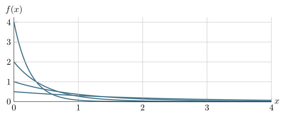
Graphs of \(\operatorname{Exponential}(0.5)\), \(\operatorname{Exponential}(1.0)\), \(\operatorname{Exponential}(2.0)\) and \(\operatorname{Exponential}(4.0)\) PDFs can be seen in the following figure:

Expected Value and Variance:

\[\begin{aligned} \operatorname{E}\!\left(X\right)= & \int_{-\infty}^{\infty}x\lambda e^{-\lambda x}dx \\ = & \int_{0}^{\infty}x\lambda e^{-\lambda x}dx \\ = & \lambda \int_{0}^{\infty}\underbrace{x}_{u}\underbrace{e^{-\lambda x}dx}_{dv} \\ \end{aligned}\]

\[\begin{aligned} u= & x \\ du= & dx \\ dv= & e^{-\lambda x}dx \\ v= & -\frac{1}{\lambda}e^{-\lambda x} \\ \end{aligned}\]

\[\begin{aligned} \operatorname{E}\!\left(X\right)= & -\left.\frac{x}{\lambda}e^{-\lambda x}\right|_{0}^{\infty}+\frac{1}{\lambda}\int_{0}^{\infty}e^{-\lambda x}dx \\ = & 0+\frac{1}{\lambda}\int_{0}^{\infty}e^{-\lambda x}dx \\ = & \frac{1}{\lambda}\left(-\left.\frac{1}{\lambda} e^{-\lambda x}\right|_{0} ^{\infty}\right) \\ = & \frac{1}{\lambda^{2}} \\ \text{So, } \operatorname{E}\!\left(X\right)= & \lambda\frac{1}{\lambda^{2}}=\frac{1}{\lambda} \end{aligned}\]

\[\begin{aligned} \operatorname{E}\!\left(X^2\right)= & \int_{0}^{\infty}x^{2}\lambda e^{-\lambda x}dx \\ = & \lambda \int_{0}^{\infty}\underbrace{x^{2}}_{u}\underbrace{e^{-\lambda xdx}}_{dv} \\ \end{aligned}\]

\[\begin{aligned} u= & x^{2} \\ du= & 2xdx \\ dv= & e^{-\lambda x}dx \\ v= & -\frac{1}{\lambda}e^{-\lambda x} \\ \end{aligned}\]

\[\begin{aligned} \operatorname{E}\!\left(X^2\right)= & \not \lambda \left[-\left.\frac{x^{2}}{\not \lambda}e^{-\lambda x}\right|_{0}^{\infty}+\frac{2}{\not \lambda} \int_{0}^{\infty} x e^{-\lambda x} d x\right] \\ = & 2 \int_{0}^{\infty}xe^{-\lambda x}dx \\ = & \frac{2}{\lambda^{2}} \\ \end{aligned}\]

\[\begin{aligned} \operatorname{Var}\left(X\right)= & \operatorname{E}\!\left(X^2\right)-(\operatorname{E}\!\left(X\right))^2 \\ = & \frac{2}{\lambda^{2}}-\frac{1}{\lambda^{2}} \\ = & \frac{1}{\lambda^{2}} \end{aligned}\]

To gain some computational insight, consider the completion of a repetitive/routine task by an office employee. Suppose that every repetition of a task takes a random duration which is governed by an \(\operatorname{Exponential}(1/4)\) distribution. As \(\lambda=1/4\), one task is, on average, completed in \(4\) time units (let’s say, days). Using this information, let’s calculate the following:

What is the probability that a task will be completed in exactly \(2\) days?
The answer here is \(0\), as time (\(X\)) here is a continuous random variable.
What is the probability that a task will be completed within \(2\) days? \[X \sim \operatorname{Exponential}(1/4)\] \[\begin{aligned} f\!\left(x\right) & =\frac{1}{4} e^{-\frac{1}{4} x}, x>0 \\ F\!\left(x\right) & =1-e^{-\frac{1}{4} x}, x>0 \\ \operatorname{P}\!\left(x \leq 2\right)=F\!\left(2\right) & =1-e^{-\frac{1}{4} \cdot 2} \\ & =0.3934 \end{aligned}\]
What is the probability that a task will be completed within \(4\) days? \[X \sim \operatorname{Exponential}(1/4)\] \[\begin{aligned} f\!\left(x\right) & =\frac{1}{4} e^{-\frac{1}{4} x}, x>0 \\ F\!\left(x\right) & =1-e^{-\frac{1}{4} x}, x>0 \\ \operatorname{P}\!\left(x \leq 4\right)=F\!\left(4\right) & =1-e^{-\frac{1}{4} \cdot 4} \\ & =0.6321 \end{aligned}\]
What is the probability that a task will be completed within \(6\) days? \[X \sim \operatorname{Exponential}(1/4)\] \[\begin{aligned} f\!\left(x\right) & =\frac{1}{4} e^{-\frac{1}{4} x}, x>0 \\ F\!\left(x\right) & =1-e^{-\frac{1}{4} x}, x>0 \\ \operatorname{P}\!\left(x \leq 6\right)=F\!\left(6\right) & =1-e^{-\frac{1}{4} \cdot 6} \\ & =0.7768 \end{aligned}\]
What is the probability that a task will be completed between \(2\) and \(6\) days? \[X \sim \operatorname{Exponential}(1/4)\] \[\begin{aligned} f\!\left(x\right) & =\frac{1}{4} e^{-\frac{1}{4} x}, x>0 \\ F\!\left(x\right) & =1-e^{-\frac{1}{4} x}, x>0 \\ \operatorname{P}\!\left(2 \leq x \leq 6\right)=F\!\left(6\right)-F\!\left(2\right) & =0.7768-0.3934 \\ & =0.3834 \end{aligned}\]

In a nutshell

Memoryless (no memory) property of Exponential distribution

A watch repairer’s repair times \(X\) follow an \(\operatorname{Exponential}(\lambda)\) distribution (where \(\lambda\) is the typical/average number of repairs per unit time). \[X \sim \operatorname{Exponential}(\lambda)\] \[\begin{aligned} & f\!\left(x\right)=\lambda e^{-\lambda x}, x>0 \\ & F\!\left(x\right)=1-e^{-\lambda x}, x>0 \end{aligned}\] At time \(0\), I left my watch for a repair and after waiting for \(T_{1}\) time units I observed that my watch was not repaired. What is the probability that I will wait for an additional (extra) \(T_{2}\) time units? A careful examination will reveal the followino: as \(T_{1}\) units of time has already passed, total waiting time will be at least \(T_{1}\), i.e., \(x>T_{1}\) will hold. This is nothing but a condition imposed on my full sample space of \(x>0\). Based on this, the original question turns into "beginning at \(T_{1}\), what is the probability that I will wait until \(T_{1}+T_{2}\)?" In technical notation, the answer is: \[\begin{aligned} & \frac{\operatorname{P}\!\left(T_{1}<x<T_{1}+T_{2}\right)}{\operatorname{P}\!\left(T_{1}<x\right)} \\ = & \frac{F\!\left(T_{1}+T_{2}\right)-F\!\left(T_{1}\right)}{1-F\!\left(T_{1}\right)} \\ = & \frac{1-e^{-\lambda\left(T_{1}+T_{2}\right)}-\left(1-e^{-\lambda T_{1}}\right)}{1-\left(1-e^{-\lambda T_{1}}\right)} \\ = & \frac{e^{-\lambda T_{1}}-e^{-\lambda\left(T_{1}+T_{2}\right)}}{e^{-\lambda T_{1}}} \\ = & e^{-\lambda T_{1}+\lambda T_{1}}-e^{-\lambda T_{1}-\lambda T_{2}+\lambda T_{1}} \\ = & e^{0}-e^{-\lambda T_{2}} \\ = & 1-e^{-\lambda T_{2}} \end{aligned}\] Now, we notice that the final expression is just equal to \(F\!\left(T_{2}\right)\), i.e., \(\operatorname{P}\!\left(x<T_{2}\right)\). \(T_{1}\) simply drops out of the solution and "probability of waiting for an additional \(T_{2}\) upon \(T_{1}\)" is equal to "probability of waiting until \(T_{2}\) at time \(0\)". Disappearance of \(T_{1}\) (or its irrelevance) implies that the random process (random variable \(X\) here) does not remember its past. This is called the memoryless (no memory) property. Drawings and graphs will be covered in the lectures.

Simulation guide

Suppose we want to simulate and analyze the purchasing decisions of \(1000\) customers arriving at a store. In such a simulation, the very first step is to create/generate these \(1000\) customers. Under certain conditions (research for them), we can (and most of the time we should) assume that arrivals of customers follow a \(\operatorname{Poisson}(\lambda\) ) distribution; so, interarrival times of the same customers follow an \(\operatorname{Exponential}(\lambda)\) distribution (which makes our lives quite easy).

The technique we use is called the "inverse transformation technique" and utilizes the inverse CDF, i.e., \(F^{-1}(x)\). The steps are:

Generate a sequence of uniform \((0,1)\) random values, call these values \(u\).
Find the \(F^{-1}(\cdot)\) expression, i.e., derive the inverse \(CDF\).
Input \(u\) into \(F^{-1}(\cdot)\) to obtain a sequence of \(x\) values. These \(x\) values are the randomly generated numbers obeying/following \(F\!\left(\cdot\right)\).

In our case of generating \(\operatorname{Exponential}(\lambda)\) interatrival times: \[\operatorname{P}\!\left(X<x\right)=F\!\left(x\right)=u, 0 \leq u \leq 1 .\] So, \[x=F^{-1}(u)\] where \[F^{-1}(u)=-\frac{\ln (1-u)}{\lambda}\] Accumulating the generated \(x\) (interarrival time) values, we can easily see the arrival times of our simulated customers. As the interarrival times have been randomly generated, arrival times are also random.

Think: What is the role and importance of \(\operatorname{Uniform}(0,1)\) distribution here?

Think: Can you use this technique to generate random values that obey another statistical distribution?

Normal distribution

\[X \sim Normal \left(\mu, \sigma^2\right)\] \[\forall x \in \mathbb{R}, f\!\left(x\right) = \frac{1}{\sqrt{2 \pi \sigma^2}} \mathrm{e} ^{-\frac{1}{2}\frac{\left(x - \mu\right)^2}{\sigma^2}}, -\infty < x < \infty\]

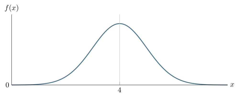
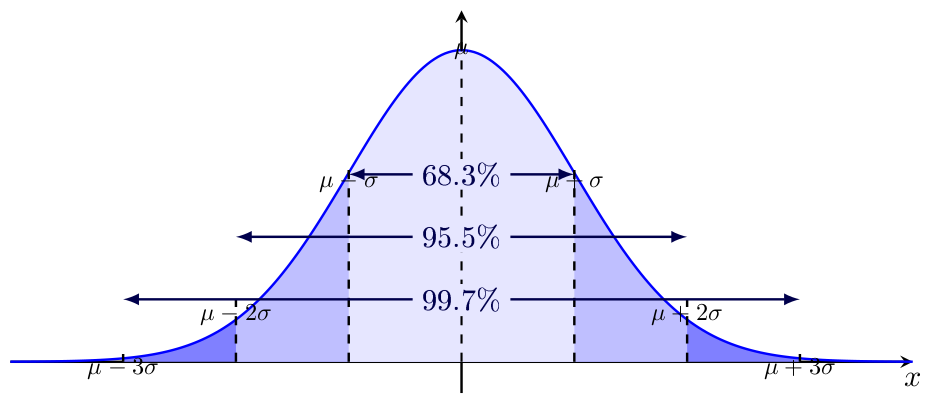
Below given the graph of \(\operatorname{Normal}(4,1)\) PDF:

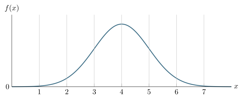
When we add the guidelines that show \(\mu-3\sigma\), \(\mu-2\sigma\), \(\mu-\sigma\), \(\mu+\sigma\), \(\mu+2\sigma\) and \(\mu+3\sigma\), the previous figure looks like:

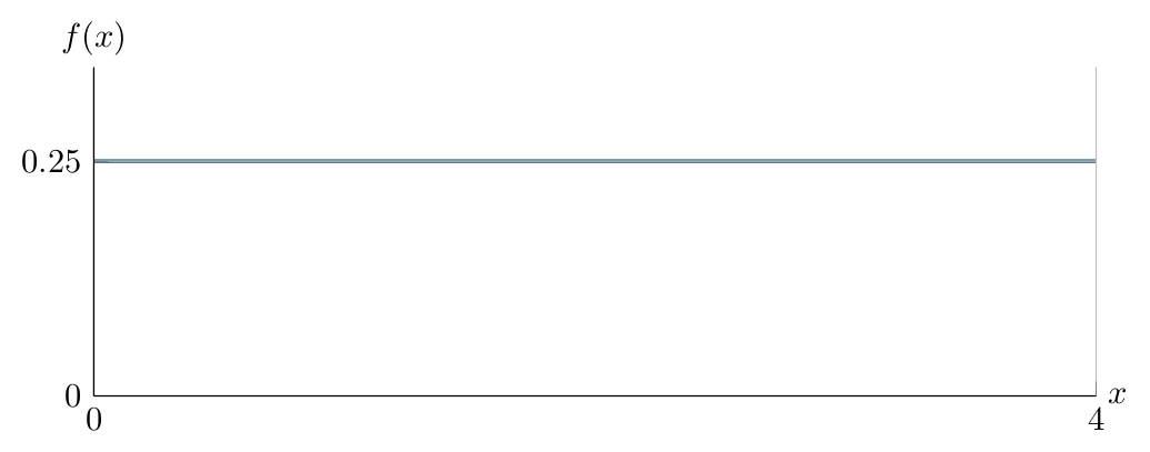
Displaying the PDFs of \(\operatorname{Normal}(4,1)\) and \(\operatorname{Normal}(4,0.25)\) together, we notice that the latter has a higher peak:

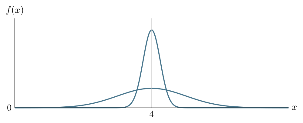
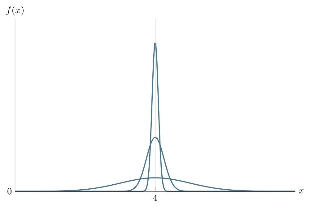
Displaying the PDFs of \(\operatorname{Normal}(4,1)\), \(\operatorname{Normal}(4,0.25)\) and \(\operatorname{Normal}(4,0.09)\) together, we notice that the last has an even higher peak, the area under each PDF integrating to \(1\).

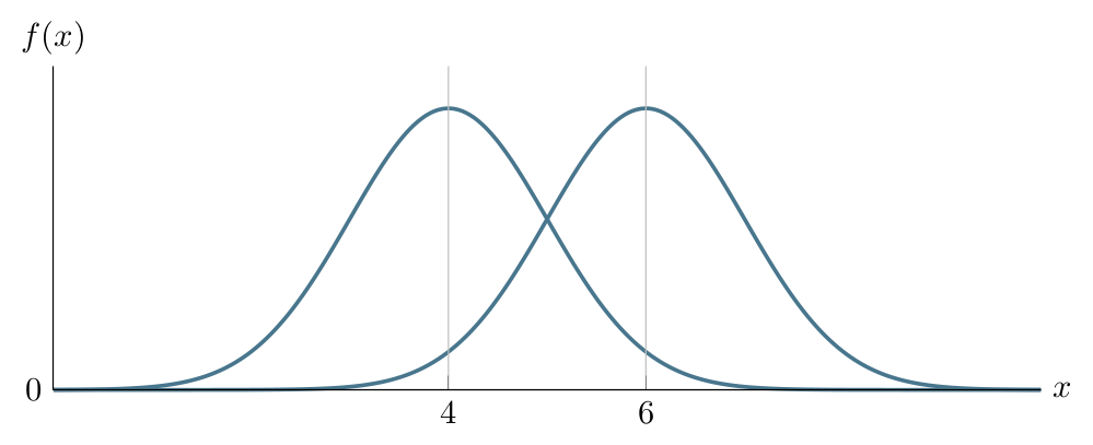
Keeping the variance \(\sigma^2\) the same, a change in mean \(\mu\) results in a shift of the PDF. Compare \(\operatorname{Normal}(4,1)\) and \(\operatorname{Normal}(6,1)\) below:

Expected Value and Variance:

\[\begin{aligned} \operatorname{E}\!\left(X\right)=\int_{-\infty}^{\infty}x\frac{1}{\sqrt{2\pi\sigma^{2}}}e^{-\frac{(x-\mu)^{2}}{2\sigma^{2}}}dx \\ \end{aligned}\]

\[\begin{aligned} z= & \frac{x-\mu}{\sigma} \\ x= & \sigma z+\mu \\ dx= & \sigma dz \\ \end{aligned}\]

\[\begin{aligned} \operatorname{E}\!\left(X\right)= & \frac{1}{\sqrt{2\pi\sigma^{2}}}\int_{-\infty}^{\infty}\left(\sigma z+\mu\right)e^{-\frac{z^{2}}{2}}\sigma dz \\ = & \frac{1}{\sqrt{2\pi}\sigma^{2}}\int_{-\infty}^{\infty}\left(\sigma^{2} z+\sigma\mu\right)e^{-\frac{z^{2}}{2}}dz \\ = & \underbrace{\frac{\sigma}{\sqrt{2 \pi}}\int_{-\infty}^{\infty}{ze^{-\frac{z^{2}}{2}}dz}}_{0}+\frac{\mu}{\sqrt{2 \pi}}\underbrace{\int_{-\infty}^{\infty}e^{-\frac{z^{2}}{2}}dz}_{\sqrt{2\pi}} \\ = & 0+\frac{\mu}{\sqrt{2\pi}}\sqrt{2\pi} \\ = & \mu \\ \end{aligned}\]

\[\begin{aligned} \operatorname{E}\!\left(X^2\right)= & \int_{-\infty}^{\infty}x^{2}\frac{1}{\sqrt{2\pi\sigma^{2}}}e^{-\frac{(x-\mu)^{2}}{2\sigma^{2}}}dx \\ \end{aligned}\]

\[\begin{aligned} z= & \frac{x-\mu}{\sigma} \\ x= & \sigma z+\mu \\ dx= & \sigma dz \\ \end{aligned}\]

\[\begin{aligned} \operatorname{E}\!\left(X^2\right)= & \frac{1}{\sqrt{2\pi\sigma^{2}}}\int_{-\infty}^{\infty}(\sigma z+\mu)^{2}e^{-\frac{z^{2}}{2}}\sigma dz \\ = & \frac{1}{\sqrt{2\pi\sigma^{2}}}\int_{-\infty}^{\infty}(\sigma^{2} z^{2}+2\sigma\mu z+\mu^{2})\sigma e^{-\frac{z^{2}}{2}}dz \\ = & \frac{\sigma^{3}}{\sqrt{2\pi\sigma^{2}}}\int_{-\infty}^{\infty}z^{2}e^{-\frac{z^{2}}{2}}dz+\frac{2\sigma^{2}\mu}{\sqrt{2\pi\sigma^{2}}}\int_{-\infty}^{\infty}ze^{-\frac{z^{2}}{2}}dz+\frac{\mu^{2}\sigma}{\sqrt{2\pi \sigma^{2}}}\int_{-\infty}^{\infty}e^{-\frac{z^{2}}{2}}dz \\ = & \frac{\sigma^{2}}{\sqrt{2 \pi}} \int_{-\infty}^{\infty} z^{2} e^{-\frac{z^{2}}{2}}dz+\frac{2\sigma\mu}{\sqrt{2\pi}}\int_{-\infty}^{\infty}z e^{-\frac{z^{2}}{2}}dz+\frac{\mu^{2}}{\sqrt{2 \pi}}\sqrt{2\pi} \\ \end{aligned}\]

\[\begin{aligned} \operatorname{E}\!\left(X^2\right)= & \frac{\sigma^{2}}{\sqrt{2\pi}}\sqrt{2\pi}+0+\mu^{2} \\ = & \sigma^{2}+\mu^{2} \\ \end{aligned}\]

\[\begin{aligned} \operatorname{Var}\left(X\right)= & \operatorname{E}\!\left(X^2\right)-(\operatorname{E}\!\left(X\right))^2 \\ = & \sigma^{2}+\mu^{2}-\mu^{2} \\ = & \sigma^{2} \end{aligned}\]

Consider \(\int_{-\infty}^{\infty} z^{2} e^{-\frac{z^{2}}{2}}dz\). For \(\alpha=\frac{1}{2}\):

\[\begin{aligned} \int_{-\infty}^{\infty}z^{2}e^{-\frac{z^{2}}{2}}dz= & \int_{-\infty}^{\infty} z^{2}e^{-\alpha z^{2}}dz \\ = & -\int_{-\infty}^{\infty}\frac{d}{d\alpha}e^{-\alpha z^{2}}dz \\ = & -\frac{d}{d\alpha}\int_{-\infty}^{\infty}e^{-\alpha z^{2}}dz \end{aligned}\]

Set \(\omega=\frac{z}{\sqrt{2\alpha}}\):

\[\begin{aligned} \int_{-\infty}^{\infty}e^{-\alpha z^{2}}dz= & \frac{1}{\sqrt{2 \alpha}} \underbrace{\int_{-\infty}^{\infty} e^{-\frac{\omega^{2}}{2}}d\omega}_{\sqrt{2\pi}} \\ = & -\frac{d}{d\alpha}\sqrt{\frac{\pi}{\alpha}} \\ = & -\sqrt{\pi}\frac{d}{d\alpha}\alpha^{-1/2} \\ = & \frac{\sqrt{\pi}}{2}\alpha^{-3/2} \\ = & \frac{\sqrt{\pi}}{2}\left(\frac{1}{2}\right)^{-3/2} \\ = & \frac{\sqrt{\pi}}{2}2^{3/2} \\ = & \sqrt{2\pi} \end{aligned}\]

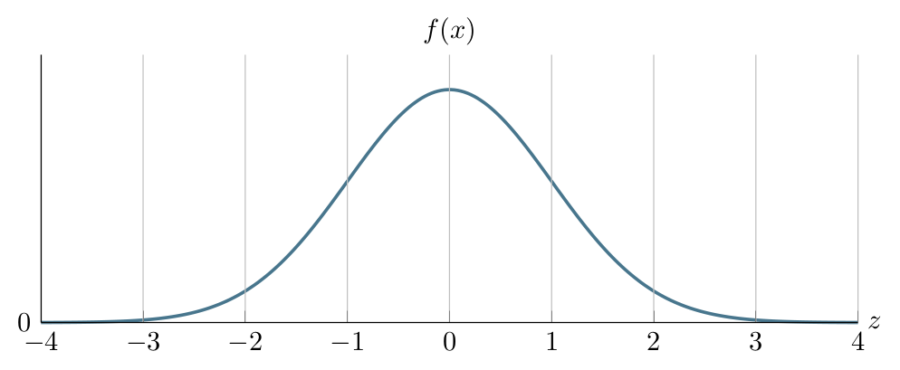
Standard normal distribution

\(Z \sim Normal \left(0, 1\right)\) has the standard normal distribution. If \(X \sim Normal \left(\mu, \sigma ^2\right)\), the random variable \(Z\) defined as: \[Z = \frac{X - \mu}{\sigma}\] has a \(\operatorname{Normal}(0,1)\) distribution. A casual naming is z-distribution, and \[f\!\left(z\right) = \frac{1}{\sqrt{2 \pi}}\mathrm{e}^{-\frac{1}{2}z^2}, -\infty < z < \infty\] Recall that, \(\mathrm{e}\) is called the Euler’s Number where \(\mathrm{e} = 2.71828\ldots\) and \(\pi = 3.14159\ldots\)

Notice/recall that the PDF of the Standard Normal (\(Z\)) random variable has a unique parametrization. Its PDF with the guidelines that show \(\mu-3\sigma=-3\), \(\mu-2\sigma=-2\), \(\mu-\sigma=-1\), \(\mu=0\), \(\mu+\sigma=1\), \(\mu+2\sigma=2\) and \(\mu+3\sigma=3\) look like:

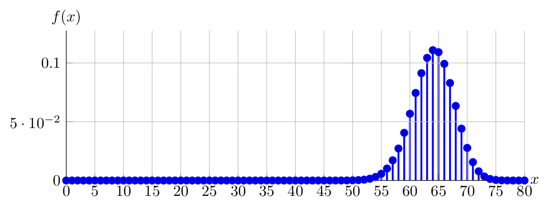
To see how/why the Normal approximation to Binomial works, consider the PDF of \(X \sim \operatorname{Binomial}(80,0.80)\) over the domains of \(0,1,\ldots,80\) and \(55,56,\ldots,75\) below:

PDF of \(X \sim \operatorname{Binomial}(80,0.80)\) plotted over \(0,1,\ldots,80\) looks like:

PDF of \(X \sim \operatorname{Binomial}(80,0.80)\) plotted over \(55,56,\ldots,75\) looks like:

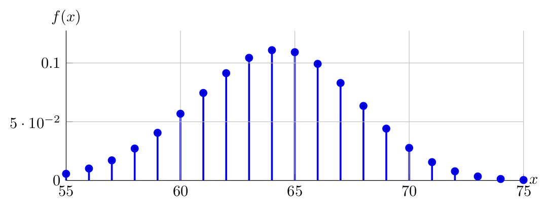
Do you see the Normal-like behavior of \(X \sim \operatorname{Binomial}(80,0.80)\) around its mean, i.e., \(nP=80\cdot0.80=64\)? Can you obtain the same with \(X \sim \operatorname{Binomial}(8,0.80)\)? Why?

Random variables and distributions: Moments of distributions [Optional material]

For each integer \(k\), the \(k^{th}\) moment of \(X\) is denoted as \(\mu_{K}^{'}\) and is defined as: \[\mu_{K}^{'} = \operatorname{E}\!\left(X^{k}\right)\] The \(k^{th}\) central moment of \(X\) is denoted as \(\mu_{k}\) and is defined as: \[\mu_{K} = \operatorname{E}\!\left(\left(X-\mu\right)^{k}\right)\] Notice that \(\mu = \mu_{1}^{'} = \operatorname{E}\!\left(X\right)\) In addition to the mean (expected value) of a random variable, another important moment is the second central moment, as you’ve known as variance.

Moment generating functions [Optional material]

\(X\) being a random variable with CDF \(F\!\left(x\right)\), the moment generating function (MGF) of \(X\) is denoted by \(M_{X}\left(t\right)\) and is defined as: \[M_{X}\left(t\right) = \operatorname{E}\!\left(\mathrm{e}^{tX}\right)\] provided that the expected value exists for \(t\) in some neighborhood of zero. That is, there exists \(h >0\) such that for all \(-h<t<h\), \(\operatorname{E}\!\left(\mathrm{e}^{eX}\right)\) exists. Otherwise, the MGF is said not to exist. Explicitly, \[M_{X}\left(t\right) = \int_{-\infty}^{\infty} \mathrm{e}^{tX} f\!\left(x\right)dx, \textit{continuous X}\] or \[M_{X}\left(t\right) = \sum_{x} \mathrm{e}^{tX} f\!\left(x\right)dx, \textit{discrete X}\]

Moment generating functions for selected distributions [Optional material]

Distribution	\(M_{X}\left(t\right)\)
\(\operatorname{Bernoulli}(p)\)	\(\left(1-p\right) + p\mathrm{e}^{t}\)
\(\operatorname{Binomial}(n,p)\)	\(\left(\left(1-p\right) + p\mathrm{e}^{t}\right)^{n}\)
\(\operatorname{Poisson}(\lambda)\)	\(\mathrm{e}^{\lambda\left(\mathrm{e}^{t}-1\right)}\)
\(\chi^2_{n}\)	\(\left(\frac{1}{1-2t}\right)^{\frac{n}{2}},\ t<\frac{1}{2}\)
\(\operatorname{Exponential}(\lambda)\)	\(\frac{1}{1-\frac{t}{\lambda}},\ t<\lambda\)
\(F_{n_{1}, n_{2}}\)	Does not exist
\(\operatorname{Normal}(\mu,\sigma^2)\)	\(\mathrm{e}^{\mu t + \frac{\sigma^2 t^2}{2}}\)
\(t_{n}\)	Does not exist
\(\operatorname{Uniform}(a,b)\)	\(\frac{\mathrm{e}^{bt} - \mathrm{e}^{at}}{\left(b-a\right)t}\)

If a random variable \(X\) has the MGF \(M_{X}\left(t\right)\), then \[\operatorname{E}\!\left(X^{n}\right) = \frac{d^{n}}{dt^{n}}M_{X}\left(t\right|_{t=0}\] That is, the \(n^{th}\) moment of \(X\) is equal to the \(n^{th}\) derivative of \(M_{X}\left(t\right)\) evaluated at \(t=0\). See after five years: convergence of MGF’s.

Exercise. We roll a pair of fair dice. Let \(X\) be the random variable that assigns the minimum of the two numbers that turn up to each outcome.

Tabulate the probability density function and cumulative distribution function of \(X\). If we know that one of the dice turned up a number less than or equal to \(3\), what is the probability that \(X\) takes a value greater than or equal to \(2\)? If we know that one of the dice turned up a number less that or equal to \(3\), what is the probability that \(X\) takes a value equal to \(3\)? Find the expected value of \(X\). Find the variance of \(X\).

Solution.

PDF is tabulated as follows:

\(x\) \(f\!\left(x\right)\)

\(1\) \(\frac{11}{36}\)

\(2\) \(\frac{9}{36}\)

\(3\) \(\frac{7}{36}\)

\(4\) \(\frac{5}{36}\)

\(5\) \(\frac{3}{36}\)

\(6\) \(\frac{1}{36}\)

This is a conditional probability question that you already are familiar with.

This is a conditional probability question that you already are familiar with.

\[\begin{aligned} \operatorname{E}\!\left(X\right) &= \sum_{x} x f\!\left(x\right) \\ &= 1 \cdot \frac{11}{36} + 2 \cdot \frac{9}{36} + 3 \cdot \frac{7}{36} + 4 \cdot \frac{5}{36} + 5 \cdot \frac{3}{36} + 6 \cdot \frac{1}{36} \\ &= \frac{11+18+21+20+15+6}{36} \\ &= \frac{91}{36} = 2.53 \end{aligned}\]

\[\begin{aligned} \operatorname{Var}\left(X\right) &= \sum_{x} \left(x-\operatorname{E}\!\left(X\right)\right)^{2} f\!\left(x\right) \\ &= \left(1-2.53\right)^{2} \cdot \frac{11}{36} + \cdots + \left(6-2.53\right)^{2} \cdot \frac{1}{36} \\ &= 1.97 \end{aligned}\]

Two balls are simultaneously chosen (i.e.., chosen without replacement) from an urn containing \(3\) white, \(2\) black, and \(1\) red balls. You are given \(2\)TL for each white ball chosen, you have to pay \(1\)TL for each black ball chosen, and you neither pay nor receive any money for a red ball that is chosen. For example if you have chosen \(1\) white and \(1\) black ball, you net winning is \(2+ \left(-1\right) =1\) TL. Let \(X\) be the random variable that gives your net winnings.

Construct a table that shows the possible values of \(X\) and the probabilities associated with each value, i.e.., tabulate the probability density (mass) function of \(X\). Find the expected value of \(X\).

Solution.

PDF is tabulated as follows:

\(x\) \(f\!\left(x\right)\)

\(-2\) \(\frac{2}{30}\)

\(-1\) \(\frac{4}{30}\)

\(1\) \(\frac{12}{30}\)

\(2\) \(\frac{6}{30}\)

\(4\) \(\frac{6}{30}\)

\[\begin{aligned} \operatorname{E}\!\left(X\right) &= \sum_{x} x f\!\left(x\right) \\ &= (-2) \cdot \frac{2}{30} + (-1) \cdot \frac{4}{30} + 1 \cdot \frac{12}{30} + 2 \cdot \frac{6}{30} + 4 \cdot \frac{6}{30} \\ &= \frac{-4-4+12+12+24}{30} \\ &= \frac{40}{30} = 1.33 \end{aligned}\]

A class in statistics has \(20\) students. In the first midterm \(2\) students scored \(50\), \(10\) scored \(60\), \(1\) scored \(70\), \(5\) scored \(80\), and \(2\) scored \(100\). Three students are selected at random without replacement. Let \(X\) be the median score of the three students.

Tabulate the probability density function of \(X\). Find the probability of the median score being greater or equal to \(80\). Given that the median of the scores of the three students selected is greater than or equal to \(70\), what is the probability that their median is equal to \(80\)? Find the expected value and variance of \(X\).

Solution. Try on your own if you have time, and just for fun.

We have three coins such that when coin \(1\) is tossed the probability of observing a head is \(0.4\), when coin \(2\) is tossed the probability of observing a head is \(0.7\), and when coin \(3\) is tossed the probability of observing a head is \(0.2\). We first toss coin \(1\). If we observe a head we toss coin \(2\) otherwise we choose coin \(1\) or coin \(3\) at random and toss it.

What is the probability of observing a head on the second toss? Are the events of observing a head on the second toss and observing a head on the first toss independent?

Solution. This question is reserved for in-class discussions.

A fair die is rolled ten times. We are interested in the number of times \(6\) is obtained.

Given our interest, can we think of this experiment as a binomial experiment. If so describe each Bernoulli trial, i.e.. verbally describe the Bernoulli trial, state the outcome that you will call success and the probability of success in each trial. Let \(X\) be the random variable which assigns, to each outcome, the number of times \(6\) is obtained in the outcome. What is the distribution of \(X\)? With what probability will \(X\) take the value \(1\)? With what probability will \(X\) take a value greater than or equal to \(4\)?

Solution.

Success is observing a \(6\), failure is observing any of \(\left\{1,2,3,4,5\right\}\). Since the die is fair, the probability of success is \(1/6\) . \(X\) being the random variable indicating the outcome of experiment, \[f\!\left(x\right)= \begin{cases}1 / 6, & x=1 \\ 5 / 6, & x=0\end{cases}\] that is, \(X \sim\) Bernoulli \((1/6)\).

Considering the whole experiment, \(X \sim \operatorname{Binomial}(10,1 / 6)\). \[f\!\left(x\right)=\left(\begin{array}{c} 10 \\ x \end{array}\right)(1 / 6)^{x}(5 / 6)^{10-x}, x=0,1,2, \ldots, 10 .\]

\[f\!\left(1\right)=\left(\begin{array}{c} 10 \\ 1 \end{array}\right)(1 / 6)^{1}(5 / 6)^{9}=0.3230\]

\[\begin{aligned} \operatorname{P}\!\left(x \geq 4\right) & =1-f\!\left(0\right)-f\!\left(1\right)-f\!\left(2\right)-f\!\left(3\right) \\ & =0.0697 \end{aligned}\]

It is known that \(40\)% of all students of Economics are male. Independent observers note the gender of \(12\) random Economics students (a student’s gender might be noted more than once) and we count the number of males observed.

What is the probability that exactly \(2\) of the observed students are male? What is the probability that the number of male students, in the group observed, is \(5\) or less? You have been told that at least \(2\) of the students that has been observed are female. What is the probability that the number of male students, in the observed group, is \(5\) or less?

Solution.

\(X \sim \operatorname{Binomial}(12,0.40)\) \[\begin{aligned} f\!\left(2\right) & =\left(\begin{array}{c} 12 \\ 2 \end{array}\right) 0.40^{2} 0.60^{10} \\ & =0.0639 \end{aligned}\]

\(x \sim \operatorname{Binomial}(12,0.40)\) \[\begin{aligned} \operatorname{P}\!\left(X \leq 5\right) & =f\!\left(0\right)+f\!\left(1\right)+f\!\left(2\right)+f\!\left(3\right)+f\!\left(4\right)+f\!\left(5\right) \\ & =F\!\left(5\right) \\ & =0.6652 \end{aligned}\]

This question is reserved for in-class discussions.

Consider a game where a round of the game consists of rolling a fair die \(10\) times. Each time a \(1\) or \(6\) comes you win \(1\)TL.

What is the probability that you will win \(5\) TL or less, if you played this game for one round? What is the probability that you will win exactly \(5\) TL, if you played this game for one round? You have learned that two of the rolls of the die resulted with a number different than \(1\) or \(6\), but you do not know what the result of the other rolls of the die was. What is the probability that you will win more than \(5\)TL? What would your average (mean) winnings be if you played this game indefinitely?

Solution.

\(X \sim \operatorname{Binomial}(10,1 / 3)\) \[\begin{aligned} \operatorname{P}\!\left(X \leq 5\right) & =F\!\left(5\right) \\ & =0.9234 \end{aligned}\]

\(X \sim \operatorname{Binomial}(10,1 / 3)\) \[\begin{aligned} f\!\left(5\right) & =\left(\begin{array}{c} 10 \\ 5 \end{array}\right)(1 / 3)^{5}(2 / 3)^{5} \\ & =0.1366 \end{aligned}\]

This question is reserved for in-class discussions.

\(X \sim \operatorname{Binomial}(10,1/3)\) \[\begin{aligned} \operatorname{E}\!\left(X\right) & =n P=10 \cdot \frac{1}{3} \\ & =3.33 \end{aligned}\]

Based on past data, we know that, on average, \(6\) customers enter Coffee Break every \(20\) minutes.

What is the probability that at least \(2\) customers will enter Coffee Break during a given \(20\)-minute time period? Define the probability of \(k\) customers entering Coffee Break in \(20\) minutes as a mathematical function. Describe what is what in your function clearly.

Solution.

\(\quad X \sim\) Poisson (6) \(\operatorname{P}\!\left(\text{At least 2 customers}\right) = 1 - \operatorname{P}\!\left(\text{At most 1 customer}\right)\) \(=1-\frac{e^{-6} 6^{0}}{0 !}-\frac{e^{-6} 6^{1}}{1 !}=0.9826\)

\(\quad X \sim\) Poisson (6) \[f\!\left(x\right)=\frac{e^{-6} 6^{x}}{x !}, x=0,1,2, \ldots\] \(X\) being the random variable that shows the number of customers arriving every 20 minutes. The rate of arriving customers is \(\lambda=6\). \(X\) is a Poisson random variable.

On an ordinary day, on average \(3\) white and \(1\) blue cars pass through a certain cross-section of a road every \(5\) minutes.

What is the probability that \(6\) white cars will pass in a \(5\)-minute interval? What is the probability that \(6\) white cars will pass in a \(10\)-minute interval? What is the probability that \(3\) cars (blue or white) will pass in a \(5\)-minute interval?

Solution.

\(\quad W \sim \operatorname{Poisson}(3)\) \[f\!\left(6\right) = \frac{\mathrm{e}^{-3}3^{6}}{6!} = 0.0504\]

\(\quad W \sim \operatorname{Poisson}(6)\) \[f\!\left(6\right) = \frac{\mathrm{e}^{-6}6^{6}}{6!} = 0.1606\]

\[\begin{aligned} X & = W+B \\ W & \sim \operatorname{Poisson}(3) \\ B & \sim \operatorname{Poisson}(1) \end{aligned}\] As Poisson \(\lambda\)’s are additive, \(X \sim \operatorname{Poisson}(4)\). \[f\!\left(3\right) = \frac{\mathrm{e}^{-4}4^{3}}{3!} = 0.1954\]

A Hypergeometric story: In a corporation, promotion decisions for employees are made by a committee of \(5\) people. The decision making procedure has the following steps:

Each of the \(5\) writes her vote (either ’Promote’ or ’Not promote’) on a piece of paper, folds the paper twice and casts the paper into a bowl.

Another person from outside the committee randomly picks \(3\) out of the \(5\) votes. (This is a step taken to anonymize votes).

The \(3\) picked papers are opened. If the employee gets \(2\) or \(3\) votes, then she is promoted. If she gets no votes or \(1\) vote, she is not promoted.

Consider Employee \(A\) for whom the chance of a promotion is \(P\) in the eyes of each committee member. That is, each committee member has a chance of \(P\) to promote Employee \(A\). Also, preferences of committee members are independent from each other’s. Is there a chance to be accidentally or unfairly promoted (or not promoted) in this kind of scheme?

Solution. The solution involves some steps:

First, a ’Promotion’ vote being marked as Success, each committee member’s vote is a Bernoulli trial:

\[X_{i} \sim \text { Bernoulli }(P), i=1,2,3,4,5\]

Then, total votes (total of successes) (\(Y\)) is a Binomial process:

\[\begin{aligned} & Y=X_{1}+X_{2}+X_{3}+X_{4}+X_{5} \\ & Y \sim \operatorname{Binomial}(5, P), \quad y=0,1,2,3,4,5 \end{aligned}\]

Then, \(W\) being the number of ’Promotion’ votes among the final \(3\), \(W\) has a Hypergometric distribution:

\(W \sim Hypergeometric(5,Y,5-Y)\)

So,

\[\begin{aligned} & f\!\left(x_{i}\right)=\begin{cases} P, x_{i}=1 \\ 1-P, x_{i}=0 \end{cases} \\ & g(y)=\left(\begin{array}{l} 5 \\ y \end{array}\right) P^{y}(1-P)^{5-y} \\ & h(w)=\frac{\left(\begin{array}{l} y \\ w \end{array}\right)\left(\begin{array}{l} 5-y \\ 3-w \end{array}\right)}{\left(\begin{array}{l} 5 \\ 3 \end{array}\right)} \end{aligned}\]

Now, your task is to find \(g(y)\) for each value of \(y\). Then you will calculate \(h(w)\) for each different value of \(y\). At the end, you will compare Employee \(A\)’s chance to promote with and without the Step 2&3 of the promotion procedure. Note that the result may be a little surprising.

Let \(X_1\) be the random variable that gives the number of phone calls that you get between \(1\) PM and \(2\) PM. Let \(X_2\) be the random variable that gives the number of phone calls that you get between \(2\)PM and \(4\)PM. Assume that \(X_1\) is Poisson distributed with parameter \(5\) and \(X_2\) is Poisson distributed with parameter \(12\). Let \(X\) be the random variable that gives the number of phone calls that you get between \(1\)PM and \(4\)PM. Find the PDF of \(X\).

Solution. \(X_{1} \sim\) Poisson (5) and \(X_{2} \sim\) Poisson (12). \(X=X_{1}+X_{2}, X \sim\) Poisson (17). Make sure you have obtained this result by following the chapter’s instructions.

Let \(X_1\) be the random variable that gives the number of phone calls that you get between \(1\)PM and \(2\)PM. Let \(X_2\) the random variable that gives the number of phone calls that your friend gets between \(1\)PM and \(2\)PM. Assume that \(X_1\) is Poisson distributed with parameter \(\lambda_1\) and \(X_2\) is Poisson distributed with parameter \(\lambda_2\). Find the distribution of \(X=X_1+X_2\), i.e.., the PDF of the random variable that gives the total number of phone calls that you and your friend receive between \(1\)PM and \(2\)PM.

Solution. The solution method is already arailable in the chapter.

Suppose that you buy \(40\) lottery tickets. Using the Poisson approximation find the probability of having at least \(2\) winning tickets, given that the probability of any ticket being a winning ticket is \(0.02\).

Solution. This is self-study for those who are interested. Not to appear in any examination.

Let \(X\) be a random variable that is uniformly distributed over \(\left(-1, 3\right)\). Answer the following questions:

Find \(P \left(X<0\right)\) Find \(P \left(\frac{1}{2} < X<1\right)\) Find \(P \left(X > 2\right)\) What is the expected value and variance of \(X\)?

Solution.

\(X \sim \operatorname{Uniform}(-1,3)\) \[\begin{aligned} & f\!\left(x\right)=\frac{1}{3-(-1)}=\frac{1}{4},-1 \leq x \leq 3 \\ & \operatorname{P}\!\left(X<0\right)=\int_{-1}^{0} \frac{1}{4} d x=\left.\frac{x}{4}\right|_{-1} ^{0} \\ & =\frac{0}{4}-\frac{-1}{4} \\ & =1/4 \\ \end{aligned}\]

\[\begin{aligned} & \quad \operatorname{P}\!\left(1 / 2<x<1\right)=\int_{1 / 2}^{1} \frac{1}{4} dx \\ & =\left.\frac{x}{4}\right|_{1 / 2} ^{1} \\ & =\frac{1}{4}-\frac{1}{8} \\ & =1 / 8 \\ \end{aligned}\]

\[\begin{aligned} & \quad \operatorname{P}\!\left(X>2\right)=\int_{2}^{3} \frac{1}{4} d x \\ & =\left.\frac{x}{4}\right|_{2} ^{3} \\ & =\frac{3}{4}-\frac{2}{4} \\ & =1 / 4 \end{aligned}\]

\[\begin{aligned} \quad \operatorname{E}\!\left(X\right) & =\frac{-1+3}{2} \\ & =1 \\ \operatorname{Var}\left(X\right) & =\frac{(3-(-1))^{2}}{12} \\ & =\frac{16}{12} \\ & =4 / 3 \end{aligned}\]

A potato chips producer starts a promotion program in an effort to boost its sales. In that, gift tickets are placed in every \(25\) out of \(100\) chip bags in sale and the customers are required to collect two tickets to win a free soft drink. By the nature of such promotions, gift tickets are invisible from outside prior to purchase. In order to attain a probability of \(90\)% at minimum to win a soft drink, how many bags of potato chips should an average customer buy? Notes:

In case a manual solution for this problem is not feasible, you are required to provide a good mathematical formulation of the solution approach along with proper explanations.

In a real life setting it is not likely to observe a high prize ratio like \(\frac{25}{100}\). Instead, one may observe ratios even lower than \(\frac{1}{100}\).

Solution. This is to be discussed in class only along with a computer demo.

Let \(X\) be a random variable with the following PDF:

\(x\) \(-3\) \(-1\) \(0\) \(1\) \(2\) \(3\)

\(f\!\left(x\right)\) \(0.25\) \(0.10\) \(0.05\) \(0.20\) \(0.30\) \(0.10\)

Define a new random variable \(Y\) as \[Y = X^2 + 1\]

Find the PDF of \(Y\) Find the CDF of \(Y\) Find the expected value of \(Y\) and show that it is equal to \(\sum \left(x^2 +1\right) f_{X}\!\left(x\right)\), where \(f\!\left(x\right)\) is the PDF of \(X\) Find the variance of \(Y\)

Solution. This question is reserved for in-class discussions.

Let \(X\) be a random variable normally distributed with expected value of \(2\) and variance of \(9\). Answer the following questions:

Find \(\operatorname{P}\!\left(X<5.15\right)\) Find \(\operatorname{P}\!\left(X<-1\right)\) Find \(\operatorname{P}\!\left(X>4\right)\) Find \(\operatorname{P}\!\left(1.04<X<3.5\right)\)

Solution.

\[\begin{aligned} & X \sim \operatorname{Normal}(2,9) \\ & \operatorname{P}\!\left(x<5.15\right)=\operatorname{P}\!\left(\frac{x-2}{3}<\frac{5.15-2}{3}\right) \\ & =\operatorname{P}\!\left(Z<1.05\right) \\ & =0.85314 \end{aligned}\]

\[\begin{aligned} \operatorname{P}\!\left(X<-1\right) & =\operatorname{P}\!\left(\frac{x-2}{3}<\frac{-1-2}{3}\right) \\ & =\operatorname{P}\!\left(Z<-1\right) \\ & =\operatorname{P}\!\left(Z>1\right) \\ & =1-F\!\left(1\right) \\ & =1-0.84134 \\ & =0.15866 \end{aligned}\] Reveal how symmetry property is used here.

\[\begin{array}{rl} \operatorname{P}\!\left(X>4\right) & =\operatorname{P}\!\left(\frac{x-2}{3}>\frac{4-2}{3}\right) \\ & =\operatorname{P}\!\left(Z>0.66\right) \\ & =1-F\!\left(0.66\right) \\ & =1-0.74537 \\ & =0.25463 \\ \end{array}\]

\[\begin{array}{rl} & \operatorname{P}\!\left(1.04<X<3.5\right) \\ = & \operatorname{P}\!\left(\frac{1.04-2}{3}<\frac{x-2}{3}<\frac{3.5-2}{3}\right) \\ = & \operatorname{P}\!\left(-0.32<z<0.50\right) \\ = & F\!\left(0.50\right)+F\!\left(0.32\right)-1 \\ = & 0.69146+0.62552-1 \\ = & 0.31698 \end{array}\] Study this solution by drawing proper graphs of the PDF of the Standard normal distribution.

It is estimated that \(45\)% of the freshmen entering a particular college will graduate from that college in four years.

For a random sample of \(5\) entering freshmen, what is the probability that exactly \(3\) will graduate in four years? For a random sample of \(5\) entering freshmen, what is the probability that a majority (more than half) will graduate in four years? \(80\) entering freshmen are chosen at random. Find the mean and variance of the number of these \(80\) that will graduate in four years.

Solution.

\(\quad X \sim \operatorname{Binomial}(5,0.45)\) \[f\!\left(3\right)=\left(\begin{array}{l} 5 \\ 3 \end{array}\right) 0.45^{3} 0.55^{2}=0.2757\]

\(X \sim \operatorname{Binomial}(5,0.45)\) \[f\!\left(3\right)+f\!\left(4\right)+f\!\left(5\right)=0.4069\]

\(X \sim \operatorname{Binomial}(80,0.45)\) \[\begin{aligned} & \operatorname{E}\!\left(X\right)=n P=80 \cdot 0.45=36 \\ & \operatorname{Var}\left(X\right)=n \operatorname{P}\!\left(1-P\right)=80 \cdot 0.45 \cdot 0.55=19.8 \end{aligned}\]

Bags of our packed by a particular machine have weights which are normally distributed with mean of \(500\)gr and standard deviation of \(20\)gr.

What is the probability that a bag weights more than \(515\)gr or less than \(490\)gr? If \(2\)% of the bags are rejected for being underweight, what is the maximum weight for a bag to be rejected as underweight? Find an interval \(\left[l,u\right]\) symmetric around the mean and the probability of the weight of a randomly selected bag being in the interval is \(0.90\).

Solution.

\(\quad X \sim \operatorname{Normal}(500,400)\) \[\begin{aligned} & \operatorname{P}\!\left(X<490\right)+\operatorname{P}\!\left(X>515\right) \\ = & \operatorname{P}\!\left(Z<\frac{490-500}{20}\right)+\operatorname{P}\!\left(Z>\frac{515-500}{20}\right) \\ = & \operatorname{P}\!\left(Z<-0.50\right)+\operatorname{P}\!\left(Z>0.75\right) \end{aligned}\] Use your \(z\) table, the answer is \(0.30853+0.22662\), i.e., \(0.53516\).

This question is reserved for in-class discussions.

This question is reserved for in-class discussions.

\(X\) is distributed as \(Bin \left(100,0.04\right)\). Describe the steps to calculate \(\operatorname{P}\!\left(X > k\right)\) for a given \(k\) by using a Poisson approximation.

Solution. This is self-study for thase who are interested. Not to appear in any examination.

We know that the number of vampires killed by Dean in a typical fight has a \(\operatorname{Poisson}(5)\) distribution and the number of vampires killed by Sam in a typical fight has a \(\operatorname{Poisson}(3)\) distribution. Show that the total number of vampires killed in a typical fight follows a \(\operatorname{Poisson}(8)\) distribution.

Solution. The solution method is already available in the chapter.

\(X\) has a \(\operatorname{Uniform}(0,100)\) distribution. Calculate \(\operatorname{P}\!\left(33<X<67\right)\), \(\operatorname{E}\!\left(X\right)\) and \(\operatorname{Var}\left(X\right)\).

Solution. \(\quad X \sim \operatorname{Uniform}(0,100)\) \[\begin{aligned} f\!\left(x\right) & =\frac{1}{100-0}, 0 \leq x \leq 100 \\ F\!\left(x\right) & =\frac{x}{100}, 0 \leq x \leq 100 \\ \end{aligned}\]

\[\begin{aligned} \operatorname{P}\!\left(33<X<67\right) & =F\!\left(67\right)-F\!\left(33\right) \\ & =\frac{67}{100}-\frac{33}{100} \\ & =\frac{34}{100} \\ \end{aligned}\]

\[\operatorname{E}\!\left(X\right)=\frac{0+100}{2}=50\]

\[\operatorname{Var}\left(X\right)=\frac{(100-0)^{2}}{12}=833.33\]

Assume that the number of phone calls that you receive in a day is governed by a Poisson process. Answer the following questions assuming that on average you receive \(3.4\) phone calls in a day.

What is the probability that you will receive at least\(3\) phone calls in a day? Given that you have already received a phone call, what is the probability that you will receive at least\(3\) phone calls? [This part is a little annoying.]

Solution. This question is left as self-study.

The probability density function for a random variable \(X\) is defined as: \[f\!\left(x\right) = \begin{cases} 0.5x & 0<x<a \\ 0 & elsewhere \\ \end{cases}\]

Find the value of \(a\) that makes \(f\!\left(x\right)\) a well-defined probability function. Calculate \(\operatorname{E}\!\left(X\right)\) and \(\operatorname{Var}\left(X\right)\)

Solution.

\(\int_{0}^{a} 0.5 x d x=1\) \(\left.0.5 \frac{x^{2}}{2}\right|_{0} ^{a}=1\) \(a^{2}-0^{2}=4\) \(a^{2}=4\) \(a=2\). When \(a\) equals \(2\), the given \(f\!\left(x\right)\) becomes a well-defined probability (distribution) function.

\[\begin{aligned} \operatorname{E}\!\left(X\right) & =\int_{0}^{2} x 0.5 x d x \\ & =0.5 \int_{0}^{2} x^{2} d x \\ & =\left.0.5 \frac{x^{3}}{3}\right|_{0} ^{2} \\ & =4 / 3 \\ \operatorname{Var}\left(X\right) & =\int_{0}^{2}(x-4 / 3)^{2} 0.5 x d x \end{aligned}\] Try on your own.

I roll a die repeatedly. In each roll, if the outcome is \(3\), my score increases by \(1\); nothing happens otherwise. Knowing that my score was initially zero, what are the expected value and variance of my score right after the \(10000^{th}\) roll?

Solution. Reveal that this physical experiment generates a random variable \(X\) with \(X \sim \operatorname{Binomial}(10000,1 / 6)\). Then, \(\operatorname{E}\!\left(X\right)=10000 \cdot(1 / 6)=1666.7\) and \(\operatorname{Var}\left(X\right)=10000 \cdot(1 / 6) \cdot(5 / 6)=1388.9\)

Suppose that you’re in charge of marketing airline seats for a major carrier. Four days before the flight date you’ve \(16\) seats remaining on the aircraft. You know from the past experience that \(80\)% of the people that purchase tickets in this time period will actually show up for the flight.

If you sell \(20\) tickets, what is the probability that you’ll overbook the flight or have at least one empty seat? What if you sell \(18\) tickets?

Solution. This exercise is left as self-study.

A machine that produces stampings for automobile engines is malfunctioning and producing \(10\)% defectives. The defective and nondefective stampings proceed from the machine in a random manner. If the next five stampings are tested, find the probability that three of them are defective.

Solution. This question is reserved for in-class discussions.

The variance of a Poisson random variable \(X\) is known to be \(4\). Calculate manually the probability that \(X\) takes a value of at least\(2\). For ease, take \(\mathrm{e} = 3\).

Solution. \(\quad X \sim \operatorname{Poisson}(\lambda)\), \(\operatorname{Var}\left(X\right)=4\). Since for a Poisson random variable \(X\sim \operatorname{Poisson}(\lambda), \operatorname{Var}\left(X\right)=\lambda\), \(\lambda=4\) here. \[\begin{aligned} \operatorname{P}\!\left(x \geq 2\right) & =1-\operatorname{P}\!\left(x \leq 1\right) \\ & =1-f\!\left(0\right)-f\!\left(1\right) \\ & =1-\frac{3^{-4} 4^{0}}{0 !}-\frac{3^{-4} 4^{1}}{1 !} \\ & =1-\frac{1}{81}-\frac{4}{81} \\ & =\frac{76}{81} \end{aligned}\]

Median and the coefficient of variation for a random variable \(X \sim N\left(\mu, \sigma^2 \right)\) are given as \(100\) and \(0.25\), respectively. Given \(F\!\left(-0.84\right)=0.20\) for the standard normal distribution, calculate the \(80^{th}\) pecentile of \(X\).

Solution. Median of a Normal random variable is equal to \(\mu\), so \(\mu=100\). \[\begin{aligned} & CV=\frac{\sigma}{\mu} \\ & 0.25=\frac{\sigma}{100} \\ & \sigma=25 \\ & \sigma^{2}=625 \end{aligned}\] So, \(X \sim\) Normal \((100,625)\). \(F\!\left(-0.84\right)=0.20\) implies \(F\!\left(0.84\right)=1-0.20=0.80\) by the symmetry of the Standard normal distribution. Based on these, the \(80th\) percentile of \(X\) is found as: \[\begin{aligned} \operatorname{P}_{80}\!\left(X\right) & =100+0.84 \cdot 25 \\ & =121 \end{aligned}\] Self-practice this solution by drawing the Normal and Standard normal PDFs.

Find the value of \[\int_{-2}^{1} \frac{1}{\sqrt{2 \pi}} \mathrm{e}^{-\frac{1}{2}z^2}dz\] with proper explanations.

Solution. Notice that the question requires the calculation of \(F\!\left(1\right)-F\!\left(-2\right)\) for the Standard normal random variable. It is nothing but the area under the standard normal PDF from \(-2\) to \(1\). The answer is \(0.8186\).

Calculate \(P \leq 8\) for \(X \sim Bin\left(1000, 0.010\right)\) using the Normal approximation to Binomial distribution.

Solution. \(X \sim Bin(1000,0.010)\) has \(\operatorname{E}\!\left(X\right)=10\) and \(\operatorname{Var}\left(X\right)=9.9\). So, \(X\) can be approximated by \(X \sim \operatorname{Normal}(10,9.9)\). Calculation of \(\operatorname{P}\!\left(X \leq 8\right)\) is then: \[\begin{aligned} \operatorname{P}\!\left(X \leq 8\right) & =\operatorname{P}\!\left(\frac{X-10}{\sqrt{9.9}} \leq \frac{8-10}{\sqrt{9.9}}\right) \\ & =\operatorname{P}\!\left(Z \leq-0.64\right) \\ & =0.262 \end{aligned}\]

We make \(100\) independent observations from a normal population with mean \(40\) and standard deviation \(20\). Approximately, what is the probability that the mean of these observations will be less than or equal \(37\)?

Solution. Indeed, this question is an early reference to sampling distributions. Each of the 100 observations has a Normal \((40,400)\) distribution, name them as \(X_{1}, X_{2}, \ldots, X_{100}\). Try to see \(\bar{X} \sim \operatorname{Normal}(40,4)\). Calculation of \(\operatorname{P}\!\left(\bar{X} \leq 37\right)\) is then straightforward.

Suppose the PDF of a logistic random variable \(X\) is given by \[f\!\left(x\right) = \frac{\mathrm{e}^{-x}}{\left(1 + \mathrm{e}^{-x}\right)^2}, -\infty <x< \infty\] Among the many of its parametrizations, this simple function is something you are familiar from your lab work during the semester.

Find \(F\!\left(x\right)\) for the random variable \(X\) by performing the necessary calculus operations. Verify that the \(F\!\left(x\right)\) you have found possesses the properties of a CDF Using the graph of \(F\!\left(x\right)\) only, find the value of \(\operatorname{E}\!\left(X\right)\)

Solution.

\[\begin{aligned} F\!\left(x\right) & =\int_{-\infty}^{x} \frac{e^{-x}}{\left(1+e^{-x}\right)^{2}} dx \\ & =\left.\frac{1}{1+e^{-x}}\right|_{-\infty} ^{x} \\ F\!\left(x\right) & =\frac{1}{1+e^{-x}},-\infty<x<\infty \end{aligned}\]

\(F\!\left(-\infty\right)=0\), \(F\!\left(\infty\right)=1\) and \(F\!\left(\cdot\right)\) is nondecreasing. \(F\) is a proper CDF here.

Try it using WolframAlpha or GeoGebra.

The class grades after an exam has a normal distribution with a mean of \(50\) and a variance of \(144\). If a student is known to have a grade less than \(70\), what is the probability that she has received a grade between \(40\) and \(60\)?

Solution. Except for the use of conditional probatrilities, this is a trivial question. Try on your own.

An experimenter tosses a coin (with \(\operatorname{P}\!\left(Tail\right)=P\)) until obtaining \(r\) successes (tails). What is the distribution of the number of tosses (\(X\)) to get \(r\) successes? Derive its PDF. Hint: \(X=x\) can occur only if there are exactly \(r-1\) successes in the first \(x-1\) trials. When you notice the first \(x-1\) trials have a Binomial structure, the rest is trivial.

Solution. \(\operatorname{P}_{r}\!\left(x\right)=\operatorname{P}\!\left(\text{r-1 successes in the first x-1 trials}\right) \times \operatorname{P}\!\left(\text{a success at the x-th trial}\right)\). The first term is nothing but the Binomial PDF & the second term is simply \(P\). So, \[\begin{aligned} \operatorname{P}_{r}\!\left(x\right) & =\left(\begin{array}{c}x-1 \\ r-1\end{array}\right) P^{r-1}(1-P)^{x-1-(r-1)} \times P \\ & =\underbrace{\left(\begin{array}{c} x-1 \\ r-1 \end{array}\right) P^{r}(1-P)^{x-r}}, x=r, r+1, r+2, \ldots \end{aligned}\] This is the PDF of the random variable described.

Consider a random variable \(x\) with \(f\!\left(x\right)=\frac{k}{\sqrt{2 \pi}} e^{-\frac{1}{2} x^{2}}, 0 \leq x<\infty\). Notice the resemblance of this PDF of the standard Normal PDF. Though, domain of \(f\!\left(x\right)\) spans the nonnegative real numbers. What should \(k\) be to make \(f\!\left(x\right)\) a proper PDF? Plot \(f\!\left(x\right)\) using your solution for \(k\).

Solution. See the past exam questions for a solution.

\(x\)	\(f\!\left(x\right)\)
\(1\)	\(\frac{11}{36}\)
\(2\)	\(\frac{9}{36}\)
\(3\)	\(\frac{7}{36}\)
\(4\)	\(\frac{5}{36}\)
\(5\)	\(\frac{3}{36}\)
\(6\)	\(\frac{1}{36}\)

\(x\)	\(f\!\left(x\right)\)
\(-2\)	\(\frac{2}{30}\)
\(-1\)	\(\frac{4}{30}\)
\(1\)	\(\frac{12}{30}\)
\(2\)	\(\frac{6}{30}\)
\(4\)	\(\frac{6}{30}\)

\(x\)	\(-3\)	\(-1\)	\(0\)	\(1\)	\(2\)	\(3\)
\(f\!\left(x\right)\)	\(0.25\)	\(0.10\)	\(0.05\)	\(0.20\)	\(0.30\)	\(0.10\)

Random vectors [Optional material]

Earlier we have studied the bivariate probabilities, yet we haven’t described bivariate probabilities referring to random variables and distribution functions. This chapter provides a calculus-based treatment of the same topic in an attempt to complete our knowledge of the topic.

In our earlier study, we’ve discussed probability models and computation of probability for events involving one variable mostly. These were the univariate models. Now, we are diving into models that involve more than one random variable, called multivariate models. As we are talking about more than one random variables, they are best represented as an \(n\)-dimensional random vector. This random vector is a function from a sample space \(S\) into \(\mathbb{R}^{n}\), i.e.. \(n\)-dimensional Euclidean space.

Joint Distributions

Let \(\left(X,Y\right)\) be a random vector. The function \(f\!\left(x,y\right): \mathbb{R}^2 \rightarrow \mathbb{R}\) defined by \[f\!\left(x,y\right) = \operatorname{P}\!\left(X=x, Y=y\right)\] is called the joint probability distribution function or joint pdf of \(\left(X,Y\right)\) if \(X\) and \(Y\) are discrete. We denote the function as \(f_{X,Y} \left(x,y\right)\)

If \(\left(X,y\right)\) is a continuous random vector, if for every \(A \subset \mathbb{R}^2\) \[\operatorname{P}\!\left(\left(X,Y\right) \in A\right) = \iint\limits_A f\!\left(x,y\right)dxdy\] \(f\!\left(x,y\right): \mathbb{R}^2 \rightarrow \mathbb{R}\) is called a joint probability density function or joint PDF of \(\left(X,Y\right)\).

Note that the following are to hold for properly defining joint PDF’s: Discrete case: \[f_{X,Y}\!\left(x,y\right) \geq 0, \forall \left(x,y\right) \in \mathbb{R}^2\] \[\sum_{\left(x,y\right)\in \mathbb{R}^2} f_{X,Y}\!\left(x,y\right) = \operatorname{P}\!\left(\left(X,Y\right) \in \mathbb{R}^2\right) = 1\] Continuous case: \[f_{X,Y}\!\left(x,y\right) \geq 0, \forall \left(x,y\right) \in \mathbb{R}^2\] \[\int_{*\infty}^{\infty} \int_{\infty}^{\infty} f\!\left(x,y\right) dxdy = 1\]

Marginal distributions

Let \(\left(X,Y\right)\) be a discrete bivariate random vector with joint PDF \(f_{X} \left(x,y\right)\). Then, the marginal PDFs of \(X\) and \(Y\) are: \[f_{X}\!\left(x\right) = \operatorname{P}\!\left(X = x\right) = \sum_{y \in \mathbb{R}} f_{X,Y} \left(x,y\right)\] and \[f_{Y}\!\left(Y\right) = \operatorname{P}\!\left(Y = y\right) = \sum_{x \in \mathbb{R}} f_{X,Y} \left(x,y\right)\]

Let \(\left(X,Y\right)\) be a continous bivariate random vector with joint PDF \(f_{X} \left(x,y\right)\). Then, the marginal PDFs of \(X\) and \(Y\) are: \[f_{X}\!\left(x\right) = \int_{-\infty}^{\infty} f_{X,Y} \left(x,y\right), \infty <x< \infty\] and \[f_{Y}\!\left(Y\right) = \sum_{x \in \mathbb{R}} f_{X,Y} \left(x,y\right), \infty <y< \infty\]

Conditional distributions

Let \(\left(X,Y\right)\) be a discrete bivariate random vector with \(f_{X,Y}\!\left(x y\right)\), \(f_{X}\!\left(x\right)\), and \(f_{Y}\!\left(y\right)\). Then, \[f_{X|Y}\!\left(x|y\right) = \operatorname{P}\!\left(X =x\,\middle|\,Y=y\right) = \frac{f_{X,Y}\!\left(x,y\right)}{f_{Y}\!\left(y\right)}, f_{Y}\!\left(y\right) \neq 0\] and \[f_{Y|X}\!\left(y|x\right) = \operatorname{P}\!\left(Y =y\,\middle|\,X=x\right) = \frac{f_{X,Y}\!\left(x,y\right)}{f_{X}\!\left(x\right)}, f_{X}\!\left(x\right) \neq 0\]

Let \(\left(X,Y\right)\) be a continous bivariate random vector with \(f_{X,Y} \left(x y\right)\), \(f_{X}\!\left(x\right)\), and \(f_{Y}\!\left(y\right)\). Then, \[f_{X|Y}\!\left(x|y\right) = \frac{f_{X,Y}\!\left(x,y\right)}{f_{Y}\!\left(y\right)}, f_{Y}\!\left(y\right) \neq 0\] and \[f_{Y|X}\!\left(y|x\right) = \frac{f_{X,Y}\!\left(x,y\right)}{f_{X}\!\left(x\right)}, f_{X}\!\left(x\right) \neq 0\]

Independence of random variables

Let \(\left(X,Y\right)\) be a bivariate random vector with \(f_{X,Y} \left(x y\right)\), \(f_{X}\!\left(x\right)\). Then, \(X\) and \(Y\) are called independent random variables if, for every \(x \in \mathbb{R}\) and \(y \in \mathbb{R}\) \[f_{X,Y} \left(xy\right) = f_{X}\!\left(x\right)f_{Y}\!\left(y\right)\] If \(X\) and \(Y\) are independent \[f_{X|Y}\!\left(x|y\right) = \frac{f_{X,Y}\!\left(x,y\right)}{f_{Y}\!\left(y\right)} = f_{X}\!\left(x\right),\] and \[f_{Y|X}\!\left(y|x\right) = \frac{f_{X,Y}\!\left(x,y\right)}{f_{X}\!\left(x\right)} = f_{Y}\!\left(y\right),\] Notice that, except for the minor changes in notation, these definitons are the same as before.

Covariance and correlation

The covariance of \(X\) and \(Y\) is the number defined by: \[Cov\left(X,Y\right) = \sigma_{XY} = \operatorname{E}\!\left(\left(X - \mu_{X}\right)\left(Y - \mu_{Y}\right)\right)\] The correlation of \(X\) and \(Y\) is the number defined by: \[\rho\left(X,Y\right) = \frac{\sigma_{XY}}{\sigma_{X}\sigma_{Y}}\] This value is also called the correlation coefficient. Note that, \(-1 \leq \rho_{XY} \leq 1\).

For any random variables \(X\) and \(Y\), \[\begin{aligned} \sigma_{XY} & = \operatorname{E}\!\left(\left(X - \mu_{X}\right)\left(Y - \mu_{Y}\right)\right) \\ & = \operatorname{E}\!\left(XY - X\mu_{Y} - Y\mu_{X} + \mu_{X} \mu_{Y}\right) \\ & = \operatorname{E}\!\left(XY\right) - \mu_{Y}\operatorname{E}\!\left(X\right) - \mu_{Y}\operatorname{E}\!\left(Y\right) + \mu_{X} \mu_{Y} \\ & = \operatorname{E}\!\left(XY\right) - \mu_{X} \mu_{Y} - \mu_{X} \mu_{Y} + \mu_{X} \mu_{Y} \\ & = \operatorname{E}\!\left(XY\right) + \mu_{X} \mu_{Y} \end{aligned}\] So, \[\sigma_{XY} = \operatorname{E}\!\left(XY\right) - \mu_{X} \mu_{Y}\]

If \(X\) and \(Y\) are independent random variables, then \[Cov \left(X,Y\right) = 0\] and \[\rho_{XY} = 0\]

Let \(X\) and \(Y\) be any two random variables, also let \(a\) and \(b\) are any two constants, then \[\operatorname{Var}\left(ax + bY\right) = a^{2} \operatorname{Var}\left(X\right) + 2ab Cov\left(X,Y\right) + b^{2}\operatorname{Var}\left(Y\right)\] or \[\sigma_{aX + bY}^{2} = a^{2} \sigma_{X}^{2} + 2ab \sigma_{XY} + b^{2} \sigma_{Y}^2\] If \(X\) and \(Y\) are independent random variables with moment generating functions \(M_{X}\left(t\right)\) and \(M_{Y}\left(t\right)\), then the moment generating function of \(X+Y\) is given by: \[M_{X + Y}\left(t\right) = M_{X}\left(t\right) M_{Y}\left(t\right)\]

Exercise.

Fill the empty cells in the tables, which are tables of joint CDF and joint PDF of the random variables \(\left(X_{1}, X_{2}\right)\).

\(f\!\left(x_{1}, x_{2}\right)\) \(0.0\) \(0.5\) \(1.0\)

\(1\) \(0.1\)

\(2\) \(0.1\)

\(3\)

\(F\!\left(x_{1}, x_{2}\right)\) \(0.0\) \(0.5\) \(1.0\)

\(1\) \(0.2\)

\(2\) \(0.5\) \(0.65\) \(0.75\)

\(3\) \(0.5\) \(0.8\)

Let \(X\) and \(Y\) be two discrete random variables with joint density function \(f\!\left(x,y\right) \in \mathbb{R}^{2}\) such that \[f\!\left(x,y\right)= \begin{cases} cxy, & x\in\left\{1,2,3\right\}\text{ and }y\in\left\{1,2\right\}, \\ 0, & \text{otherwise}. \end{cases}\]

Find the value of \(c\) Find \(\operatorname{P}\!\left(Y < X\right)\) Find \(\operatorname{P}\!\left(Y = X\right)\) Find the PDF of \(X\) and PDF of \(Y\) Find the conditional distribution of \(Y\) given \(x=1\) Are the random variables \(X\) and \(Y\) independent? Find the expected value of \(X\) Find the variance of \(X\)

First we pick a number, at random, from the interval \(\left(0,1\right)\), then we pick a number, at random, from the interval \(\left(0,x_{1}\right)\). Let \(X_1\) be the random variable that gives the value of the first number and \(X_2\) the random variable of the second number. The distribution of \(X_1\) is uniform over \(\left(0,1\right)\) and the distribution of \(X_2\) given that \(x_1 = x_1\) is uniform over \(\left(0,x_{1}\right)\)

Find the joint PDF of \(\left(X_{1}, X_{2}\right)\). Find the PDF of \(X_2\) (the second marginal distribution of \(\left(X_{1}, X_{2}\right)\)). Find the conditional distribution of \(X_1\) given \(X_2 = x_2\).