Chapter 7
Hypothesis testing
Hypothesis testing: One population
A sizable volume of scientific efforts involve questions on a given population parameter. While we estimate/calculate an interval to contain an unknown population parameter with a probability of \(\left(1-\alpha\right)100\%\) under the heading of Confidence interval estimation, here in Hypothesis testing, we question the viability of a given value as the value of our unknown population parameter.
So, what we do is to check for the validity of a claim about an unknown, in formal terms.
A statistical hypothesis is a statement about the numerical value of a parameter. The null hypothesis, denoted \(H_{0}\), represents the hypothesis that is assumed to be true unless the data provide convincing counter evidence. This usually represents the status quo or some claim about the parameter that the researcher states.
The alternative hypothesis, denoted \(H_{1}\), represents the hypothesis that will be maintained only if the data provide convincing evidence for its truth.
The test statistic is a sample statistic, computed from information provided in the sample, that the researcher uses to decide between the null and alternative hypotheses.
A Type I error occurs if the researcher rejects the null hypothesis in favor of the alternative hypothesis when, in fact, the null hypothesis is true. The probability of Type I error is denoted as \(\alpha\).
The rejection region of a statistical test is the set of possible values of the test statistic for which the researcher will reject the null hypothesis in favor of the alternative.
A Type II error occurs if the researcher fails to reject the null hypothesis when, in fact, the null hypothesis is false. The probability of Type II error is denoted as \(\beta\).
Exercise. For each of the situations below write the null and alternative hypotheses, corresponding to the test, in plain English; then write the null and alternative hypotheses using only mathematical symbols; then state what the symbols you used above represents:
We would like to test if the income share held by the highest earning \(20\%\) is less than \(46\%\). We would like to test if the average income of males is greater than the average income of females. It is claimed that, among the people who drinks at least \(2\) liters of water every day, the percentage of those with a kidney problem is less than \(5\%\). We suspect the truth of this statement and would like to test it. We would like to test if a coin is fair. We would like to test if a coin is not a fair coin.
Solution. This exercise is left as self-study.
Hypothesis testing
Mean of a normal population
Case: Known population variance
Consider:
\(H_{0}: \mu \leq \mu_{0}\)
\(H_{1}: \mu > \mu_{0}\)
and \(\left\{x_{i}\right\}_{i=1}^{n}\), a random sample of \(n\) observations from a normal population \(\operatorname{Normal}(\mu, \sigma^{2})\) with known \(\sigma^{2}\).
At the statistical significance level \(\alpha\):
\(H_{0}\) is rejected if \[\frac{\bar{x} - \mu_{0}}{\frac{\sigma}{\sqrt{n}}} > z_{1-\alpha}\]
and we fail to reject \(H_{0}\) otherwise.
Exercise. A researcher wonders if the mean wage rate of workers in Ankara is greater than \(6500\). The population variance is known to be \(1000000\). The researcher measures the mean wage rate of a sample of \(64\) workers as \(7000\). Conduct and conclude the relevant hypothesis testate the significance level of \(5\%\).
Solution.
\(H_{0}: \mu \leq 6500\)
\(H_{1}: \mu > 6500\)The relevant distribution is \(z\).
Since: \[\frac{7000 - 6500}{\frac{1000}{\sqrt{64}}} =4.00 > 1.65\] we reject \(H_{0}\) at \(\alpha=0.05\).
For:
\(H_{0}: \mu \geq \mu_{0}\)
\(H_{1}: \mu < \mu_{0}\)
At the statistical significance level \(\alpha\):
\(H_{0}\) is rejected if \[\frac{\bar{x} - \mu_{0}}{\frac{\sigma}{\sqrt{n}}} < z_{\alpha}\]
and we fail to reject \(H_{0}\) otherwise.
Exercise. A researcher wonders if the mean wage rate of workers in Ankara is less than \(7500\). The population variance is known to be \(1000000\). The researcher measures the mean wage rate of a sample of \(64\) workers as \(7000\). Conduct and conclude the relevant hypothesis testate the significance level of \(5\%\).
Solution.
\(H_{0}: \mu \geq 7500\)
\(H_{1}: \mu < 7500\)The relevant distribution is \(z\).
Since: \[\frac{7000 - 7500}{\frac{1000}{\sqrt{64}}} = -4.00 < -1.65\] we reject \(H_{0}\) at \(\alpha=0.05\).
For:
\(H_{0}: \mu = \mu_{0}\)
\(H_{1}: \mu \neq \mu_{0}\)
At the statistical significance level \(\alpha\):
\(H_{0}\) is rejected if \[\frac{\bar{x} - \mu_{0}}{\frac{\sigma}{\sqrt{n}}} < z_{\frac{\alpha}{2}} \text{ or } \frac{\bar{x} - \mu_{0}}{\frac{\sigma}{\sqrt{n}}} > z_{1-\frac{\alpha}{2}}\]
and we fail to reject \(H_{0}\) otherwise.
Exercise. A researcher wonders if the mean wage rate of workers in Ankara is different than \(7500\). The population variance is known to be \(1000000\). The researcher measures the mean wage rate of a sample of \(64\) workers as \(7000\). Conduct and conclude the relevant hypothesis testate the significance level of \(5\%\).
Solution.
\(H_{0}: \mu = 7500\)
\(H_{1}: \mu \neq 7500\)The relevant distribution is \(z\).
Since: \[\frac{7000 - 7500}{\frac{1000}{\sqrt{64}}} = -4.00 \text{ is outside of } [-1.96,1.96]\] we reject \(H_{0}\) at \(\alpha=0.05\).
Hypothesis testing
Mean of a normal population
Case: Unknown population variance
Consider:
\(H_{0}: \mu \leq \mu_{0}\)
\(H_{1}: \mu > \mu_{0}\)
and \(\left\{x_{i}\right\}_{i=1}^{n}\), a random sample of \(n\) observations from a normal population \(\operatorname{Normal}(\mu, \sigma^{2})\) where \(\sigma^{2}\) is unkown.
At the statistical significance level \(\alpha\):
\(H_{0}\) is rejected if \[\frac{\bar{x} - \mu_{0}}{\frac{s}{\sqrt{n}}} > t_{n-1,1-\alpha}\]
and we fail to reject \(H_{0}\) otherwise.
Exercise. A researcher wonders if the mean wage rate of workers in Ankara is greater than \(6500\) , for which the population variance is unknown. The researcher measures the mean wage rate of a sample of \(64\) workers as \(7000\) and the ’sample variance’ as \(640000\). Conduct and conclude the relevant hypothesis test at the significance level of \(5\%\).
Solution.
\(H_{0}: \mu \leq 6500\)
\(H_{1}: \mu > 6500\)The relevant distribution is \(t\) and the degrees of freedom is \(63\).
Since: \[\frac{7000 - 6500}{\frac{800}{\sqrt{64}}} = 5.00 > 1.669\] we reject \(H_{0}\) at \(\alpha=0.05\).
For:
\(H_{0}: \mu \geq \mu_{0}\)
\(H_{1}: \mu < \mu_{0}\)
At the statistical significance level \(\alpha\):
\(H_{0}\) is rejected if \[\frac{\bar{x} - \mu_{0}}{\frac{s}{\sqrt{n}}} < t_{n-1,\alpha}\]
and we fail to reject \(H_{0}\) otherwise.
Exercise. A researcher wonders if the mean wage rate of workers in Ankara is less than \(7500\) , for which the population variance is unknown. The researcher measures the mean wage rate of a sample of \(64\) workers as \(7000\) and the ’sample variance’ as \(640000\). Conduct and conclude the relevant hypothesis test at the significance level of \(5\%\).
Solution.
\(H_{0}: \mu \geq 7500\)
\(H_{1}: \mu < 7500\)The relevant distribution is \(t\) and the degrees of freedom is \(63\).
Since: \[\frac{7000 - 7500}{\frac{800}{\sqrt{64}}} = -5.00 < -1.669\] we reject \(H_{0}\) at \(\alpha=0.05\).
For:
\(H_{0}: \mu = \mu_{0}\)
\(H_{1}: \mu \neq \mu_{0}\)
At the statistical significance level \(\alpha\):
\(H_{0}\) is rejected if \[\frac{\bar{x} - \mu_{0}}{\frac{s}{\sqrt{n}}} < t_{n-1,\frac{\alpha}{2}} \text{ or } \frac{\bar{x} - \mu_{0}}{\frac{s}{\sqrt{n}}} > t_{n-1,1-\frac{\alpha}{2}}\]
and we fail to reject \(H_{0}\) otherwise.
Exercise. A researcher wonders if the mean wage rate of workers in Ankara is different than \(7500\) , for which the population variance is unknown. The researcher measures the mean wage rate of a sample of \(64\) workers as \(7000\) and the ’sample variance’ as \(640000\). Conduct and conclude the relevant hypothesis test at the significance level of \(5\%\).
Solution.
\(H_{0}: \mu = 7500\)
\(H_{1}: \mu \neq 7500\)The relevant distribution is \(t\) and the degrees of freedom is \(63\).
Since: \[\frac{7000 - 7500}{\frac{800}{\sqrt{64}}} = -5.00 \text{ is outside of } [-1.998,1.998]\] we reject \(H_{0}\) at \(\alpha=0.05\).
Hypothesis testing
Population proportion
Consider:
\(H_{0}: P \leq P_{0}\)
\(H_{1}: P > P_{0}\)
and \(\left\{x_{i}\right\}_{i=1}^{n}\), a random sample of \(n\) observations from a \(\operatorname{Bernoulli}(P)\) population.
At the statistical significance level \(\alpha\):
\(H_{0}\) is rejected if \[\frac{\hat{p} - P_{0}}{\sqrt{\frac{\operatorname{P}_{0}\!\left(1-P_{0}\right)}{n}}} > z_{1-\alpha}\]
and we fail to reject \(H_{0}\) otherwise.
Exercise. A political candidate wonders if her nationwide support rate exceeds \(50\%\). Among a sample of \(64\) people, we know \(35\) support the political candidate. Conduct and conclude the relevant hypothesis test at the significance level of \(5\%\).
Solution.
\(H_{0}: P \leq 0.50\)
\(H_{1}: P > 0.50\)The relevant distribution is \(z\).
Since: \[\frac{0.547 - 0.500}{\sqrt{\frac{0.500 \left(1 - 0.500 \right)}{64}}} = 0.750 \text{ is not greater than } 1.65\] we fail to reject \(H_{0}\) at \(\alpha=0.05\).
For:
\(H_{0}: P \geq P_{0}\)
\(H_{1}: P < P_{0}\)
At the statistical significance level \(\alpha\):
\(H_{0}\) is rejected if \[\frac{\hat{p} - P_{0}}{\sqrt{\frac{\operatorname{P}_{0}\!\left(1-P_{0}\right)}{n}}} < z_{\alpha}\]
and we fail to reject \(H_{0}\) otherwise.
Exercise. A political candidate wonders if her nationwide support rate falls short of \(50\%\). Among a sample of \(64\) people, we know \(30\) support the political candidate. Conduct and conclude the relevant hypothesis test at the significance level of \(5\%\).
Solution.
\(H_{0}: P \geq 0.50\)
\(H_{1}: P < 0.50\)The relevant distribution is \(z\).
Since: \[\frac{0.469 - 0.500}{\sqrt{\frac{0.500 \left(1 - 0.500 \right)}{64}}} = -0.500 \text{ is not less than} -1.65\] we fail to reject \(H_{0}\) at \(\alpha=0.05\).
For:
\(H_{0}: P = P_{0}\)
\(H_{1}: P \neq P_{0}\)
At the statistical significance level \(\alpha\):
\(H_{0}\) is rejected if \[\frac{\hat{p} - P_{0}}{\sqrt{\frac{\operatorname{P}_{0}\!\left(1-P_{0}\right)}{n}}} < z_{\frac{\alpha}{2}} \text{ or } \frac{\hat{p} - P_{0}}{\sqrt{\frac{\operatorname{P}_{0}\!\left(1-P_{0}\right)}{n}}} > z_{1-\frac{\alpha}{2}}\]
and we fail to reject \(H_{0}\) otherwise.
Exercise. A political candidate wonders if her nationwide support rate is different than \(50\%\). Among a sample of \(64\) people, we know \(35\) support the political candidate. Conduct and conclude the relevant hypothesis test at the significance level of \(5\%\).
Solution.
\(H_{0}: P = 0.50\)
\(H_{1}: P \neq 0.50\)The relevant distribution is \(z\).
Since: \[\frac{0.469 - 0.500}{\sqrt{\frac{0.500 \left(1 - 0.500 \right)}{64}}} = -0.500 \text{ is not outside } [-1.96,1.96]\] we fail to reject \(H_{0}\) at \(\alpha=0.05\).
Hypothesis testing
Variance of a normal population
Consider:
\(H_{0}: \sigma^{2} \leq \sigma_{0}^{2}\)
\(H_{1}: \sigma^{2} > \sigma_{0}^{2}\)
and \(\left\{x_{i}\right\}_{i=1}^{n}\), a random sample of \(n\) observations from a normal population \(\operatorname{Normal}(\mu, \sigma^{2})\).
At the statistical significance level \(\alpha\):
\(H_{0}\) is rejected if \[\frac{\left(n-1\right)s^{2}}{\sigma_{0}^{2}} > \chi^2_{n-1,1-\alpha}\]
and we fail to reject \(H_{0}\) otherwise.
Exercise. A process engineer is concerned with the variation of - temperature in an industrial furnace and wonders if it exceeds \(1500\). She collects a random sample of temperatures as: \[\begin{array}{rrrr} 975 & 1075 & 1050 & 900 \\ 1000 & 950 & 1025 & 1050 \\ 975^{\circ} \mathrm{C} & & & \end{array}\] Conduct and conclude the relevant hypothesis test at the significance level of \(5\%\).
Solution.
\(H_{0}: \sigma^{2} \leq 1500\)
\(H_{1}: \sigma^{2} > 1500\)The relevant distribution is \(\chi^2\) and the degrees of freedom is \(8\).
Since: \[\frac{\left(9-1\right)3125}{1500} = 16.667 > 15.507\] we reject \(H_{0}\) at \(\alpha=0.05\).
For:
\(H_{0}: \sigma^{2} \geq \sigma_{0}^{2}\)
\(H_{1}: \sigma^{2} < \sigma_{0}^{2}\)
At the statistical significance level \(\alpha\):
\(H_{0}\) is rejected if \[\frac{\left(n-1\right)s^{2}}{\sigma_{0}^{2}} < \chi^2_{n-1,\alpha}\]
and we fail to reject \(H_{0}\) otherwise.
Exercise. A process engineer is concerned with the variation of - temperature in an industrial furnace and wonders if it is less than \(2500\). She collects a random sample of temperatures as: \[\begin{array}{rrrr} 975 & 1075 & 1050 & 900 \\ 1000 & 950 & 1025 & 1050 \\ 975^{\circ} \mathrm{C} & & & \end{array}\] Conduct and conclude the relevant hypothesis test at the significance level of \(5\%\).
Solution.
\(H_{0}: \sigma^{2} \geq 2500\)
\(H_{1}: \sigma^{2} < 2500\)The relevant distribution is \(\chi^2\) and the degrees of freedom is \(8\).
Since: \[\frac{\left(9-1\right)3125}{2500} = 10.000 \text{ is not less than } 2.733\] we fail to reject \(H_{0}\) at \(\alpha=0.05\).
For:
\(H_{0}: \sigma^{2} = \sigma_{0}^{2}\)
\(H_{1}: \sigma^{2} \neq \sigma_{0}^{2}\)
At the statistical significance level \(\alpha\):
\(H_{0}\) is rejected if \[\frac{\left(n-1\right)s^{2}}{\sigma_{0}^{2}} < \chi^2_{n-1,\frac{\alpha}{2}} \text{ or } \frac{\left(n-1\right)s^{2}}{\sigma_{0}^{2}} > \chi^2_{n-1,1-\frac{\alpha}{2}}\]
and we fail to reject \(H_{0}\) otherwise.
Exercise. A process engineer is concerned with the variation of - temperature in an industrial furnace and wonders if it is different than \(2000\). She collects a random sample of temperatures as: \[\begin{array}{rrrr} 975 & 1075 & 1050 & 900 \\ 1000 & 950 & 1025 & 1050 \\ 975^{\circ} \mathrm{C} & & & \end{array}\] Conduct and conclude the relevant hypothesis test at the significance level of \(5\%\).
Solution.
\(H_{0}: \sigma^{2} = 2000\)
\(H_{1}: \sigma^{2} \neq 2000\)The relevant distribution is \(\chi^2\) and the degrees of freedom is \(8\).
Since: \[\frac{\left(9-1\right)3125}{2000} = 12.500 \text{ is not outside } [2.180,17.535]\] we fail to reject \(H_{0}\) at \(\alpha=0.05\).
Exercise. A manufacturer of automobile batteries claim that at least \(80\%\) of the batteries that it produces will last \(36\) months. A consumers’ advocate group wants to evaluate this longevity claim and selects a random sample of \(28\) batteries to test. The following data indicate the length of time (in months) that each of these batteries lasted (i.e., performed properly before failure):
\(42.3\), \(39.6\), \(25.0\), \(56.2\), \(37.2\), \(47.4\), \(57.5\), \(39.3\), \(39.2\), \(47.0\), \(47.4\), \(39.7\), \(57.3\), \(51.8\), \(31.6\), \(45.1\), \(40.8\), \(42.4\), \(38.9\), \(42.9\), \(34.1\), \(49.0\), \(41.5\), \(60.1\), \(34.6\), \(50.4\), \(30.7\), \(44.1\)
Now, we would like to test, at a significance level of \(0.05\), if there is a significant evidence that less than \(80\%\) of the batteries will last at least \(36\) months? Conduct and conclude the test.
Solution. The critical element of solution is that what we are testing here is not the mean product life, rather it is the proportion of items that last at least \(36\) months. So, begin by counting the product lifetimes (among the given \(28\) measurements), calculate \(\hat{p}\) and proceed straightforwardly with the rest. 8402 This exercise is left as self-study.
Right after the poll stations are closed at 17:00, a political candidate receives the information that out of the \(50\) people interviewed her approval "count" is \(24\). As a statistics lover, she immediately tests the null hypothesis that her population approval rate is less than or equal \(0.50\) against its respective alternative, at the \(5\%\) level of statistical significance. What is the conclusion of this test? Suppose in every consecutive \(15\) minutes, number of people interviewed increases by \(5\) and approval count increases by \(4\). Find the earliest time, HH:MM, that she can declare her victory based on her tests of hypotheses. Note that a formal statistical/algebraic solution is expected with proper terminology and notation.
Solution. This exercise is left as self-study.
Hypothesis testing: Two populations
In this part, you are more than welcome to transfer your earlier, indeed recently acquired, knowledge to understand things better. Except for one case or two, the material remains fairly intact compared to the ones in confidence intervals for two populations.
Hypothesis testing
Difference between two normal population means
Case: Dependent (matched) samples
Consider:
\(H_{0}: \mu_{x} - \mu_{y} \leq 0\)
\(H_{1}: \mu_{x} - \mu_{y} > 0\)
Let \(\left\{x_{i}\right\}_{i=1}^{n}\) and \(\left\{y_{i}\right\}_{i=1}^{n}\), be two matched samples.
At the statistical significance level \(\alpha\):
\(H_{0}\) is rejected if \[\frac{\bar{d}}{\frac{s_{d}}{\sqrt{n}}} > t_{n-1,1-\alpha}\]
and we fail to reject \(H_{0}\) otherwise.
For:
\(H_{0}: \mu_{x} - \mu_{y} \geq 0\)
\(H_{1}: \mu_{x} - \mu_{y} < 0\)
At the statistical significance level \(\alpha\):
\(H_{0}\) is rejected if \[\frac{\bar{d}}{\frac{s_{d}}{\sqrt{n}}} < t_{n-1,\alpha}\]
and we fail to reject \(H_{0}\) otherwise.
For:
\(H_{0}: \mu_{x} - \mu_{y} = 0\)
\(H_{1}: \mu_{x} - \mu_{y} \neq 0\)
At the statistical significance level \(\alpha\):
\(H_{0}\) is rejected if \[\frac{\bar{d}}{\frac{s_{d}}{\sqrt{n}}} < t_{n-1,\frac{\alpha}{2}} \text{ or } \frac{\bar{d}}{\frac{s_{d}}{\sqrt{n}}} > t_{n-1,1-\frac{\alpha}{2}}\]
and we fail to reject \(H_{0}\) otherwise.
Exercise. A company is about to release a new drug to assist weight loss, and we are in charge of assessing how effective the drug is. We pick a random sample of \(8\) people with the following pre-drug body weights: \[90, 95, 105, 95, 110, 85, 100, 90\] After using the drug for the designated test duration, the post-drug body weights are measured as: \[85, 80, 110, 90, 110, 80, 95, 90\] Conduct and conclude a hypothesis test at the significance level of \(5\%\) to assess if ’pre-drug minus post-drug difference of mean body weights is positive’.
Solution.
\(H_{0}: \mu_{x} - \mu_{y} \leq 0\)
\(H_{1}: \mu_{x} - \mu_{y} > 0\)The difference series (pre-drug minus post-drug) is: \[+5, +15, -5, +5, 0, +5, +5, 0\] The relevant distribution is \(t\) and the degrees of freedom is \(7\).
Since: \[\frac{3.75}{\frac{5.825}{\sqrt{8}}} = 1.821 \text{ is not greater than }> 1.895\] we fail to reject \(H_{0}\) at \(\alpha=0.05\).
Hypothesis testing
Difference between two normal population means
Case: Independent samples & Known population variances
Consider:
\(H_{0}: \mu_{x} - \mu_{y} \leq 0\)
\(H_{1}: \mu_{x} - \mu_{y} > 0\)
Let,
\(\left\{x_{i}\right\}_{i=1}^{n_{x}} \subset \left\{x_{i}\right\}_{i=1}^{N_{x}} \sim \operatorname{Normal}(\mu_{x}, \sigma_{x}^{2} )\) \(\left\{y_{i}\right\}_{i=1}^{n_{y}} \subset \left\{y_{i}\right\}_{i=1}^{N_{y}} \sim \operatorname{Normal}(\mu_{y}, \sigma_{y}^{2} )\)
where \(\sigma_{x}^{2}\) and \(\sigma_{y}^{2}\) are known.
At the statistical significance level \(\alpha\):
\(H_{0}\) is rejected if \[\frac{\bar{x} - \bar{y}}{\sqrt{\frac{\sigma_{x}^{2}}{n_{x}}} + \frac{\sigma_{y}^{2}}{n_{y}}} > z_{1-\alpha}\]
and we fail to reject \(H_{0}\) otherwise.
For:
\(H_{0}: \mu_{x} - \mu_{y} \geq 0\)
\(H_{1}: \mu_{x} - \mu_{y} < 0\)
At the statistical significance level \(\alpha\):
\(H_{0}\) is rejected if \[\frac{\bar{x} - \bar{y}}{\sqrt{\frac{\sigma_{x}^{2}}{n_{x}}} + \frac{\sigma_{y}^{2}}{n_{y}}} < z_{\alpha}\]
and we fail to reject \(H_{0}\) otherwise.
For:
\(H_{0}: \mu_{x} - \mu_{y} = 0\)
\(H_{1}: \mu_{x} - \mu_{y} \neq 0\)
At the statistical significance level \(\alpha\):
\(H_{0}\) is rejected if \[\frac{\bar{x} - \bar{y}}{\sqrt{\frac{\sigma_{x}^{2}}{n_{x}}} + \frac{\sigma_{y}^{2}}{n_{y}}} < z_{\frac{\alpha}{2}} \text{ or } \frac{\bar{x} - \bar{y}}{\sqrt{\frac{\sigma_{x}^{2}}{n_{x}}} + \frac{\sigma_{y}^{2}}{n_{y}}} > z_{1-\frac{\alpha}{2}}\]
and we fail to reject \(H_{0}\) otherwise.
Exercise. A researcher wonders if the mean wage of workers in Ankara falls short of that in Istanbul. She has the following data and information: Mean wage rate of \(49\) workers from Ankara is \(6000\). Mean wage rate of \(81\) workers from Istanbul is \(7000\). Population variance of wages in Ankara and Istanbul are known to be \(640000\) and \(810000\), respectively. Conduct and conclude a hypothesis test at the significance level of \(5\%\) to assess if mean wage rate in Ankara is less than the mean wage rate in Istanbul.
Solution.
\(H_{0}: \mu_{x} - \mu_{y} \geq 0\)
\(H_{1}: \mu_{x} - \mu_{y} < 0\)The relevant distribution is \(z\).
Since: \[\frac{6000 - 7000}{\sqrt{\frac{640000}{49}} + \frac{810000}{81}} = -6.585 < -1.65\] we reject \(H_{0}\) at \(\alpha=0.05\).
Hypothesis testing
Difference between two normal population means
Case: Independent samples & Unknown yet equal population variances
Consider:
\(H_{0}: \mu_{x} - \mu_{y} \leq 0\)
\(H_{1}: \mu_{x} - \mu_{y} > 0\)
Let,
\(\left\{x_{i}\right\}_{i=1}^{n_{x}} \subset \left\{x_{i}\right\}_{i=1}^{N_{x}} \sim \operatorname{Normal}(\mu_{x}, \sigma_{x}^{2} )\) \(\left\{y_{i}\right\}_{i=1}^{n_{y}} \subset \left\{y_{i}\right\}_{i=1}^{N_{y}} \sim \operatorname{Normal}(\mu_{y}, \sigma_{y}^{2} )\)
where \(\sigma_{x}^{2}\) and \(\sigma_{y}^{2}\) are unkown but assumed to be equal.
At the statistical significance level \(\alpha\):
\(H_{0}\) is rejected if \[\frac{\bar{x} - \bar{y}}{\sqrt{\frac{s_{p}^{2}}{n_{x}}} + \frac{s_{p}^{2}}{n_{y}}} > t_{n_{x} + n_{y} -2, 1-\alpha}\]
and we fail to reject \(H_{0}\) otherwise.
In our formulation: \[s_{p}^{2} = \frac{\left(n_{x} - 1\right)s_{x}^{2} + \left(n_{y} - 1\right) s_{y}^{2}}{n_{x} + n_{y} -2}\] and, \[s_{x}^{2} = \frac{\sum_{i=1}^{n_{x}} \left(x_{i} - \bar{x}\right)^{2}}{n_{x} - 1}\] \[s_{y}^{2} = \frac{\sum_{i=1}^{n_{y}} \left(y_{i} - \bar{y}\right)^{2}}{n_{y} - 1}\]
For:
\(H_{0}: \mu_{x} - \mu_{y} \geq 0\)
\(H_{1}: \mu_{x} - \mu_{y} < 0\)
At the statistical significance level \(\alpha\):
\(H_{0}\) is rejected if \[\frac{\bar{x} - \bar{y}}{\sqrt{\frac{s_{p}^{2}}{n_{x}}} + \frac{s_{p}^{2}}{n_{y}}} < t_{n_{x} + n_{y} -2, \alpha}\]
and we fail to reject \(H_{0}\) otherwise.
For:
\(H_{0}: \mu_{x} - \mu_{y} = 0\)
\(H_{1}: \mu_{x} - \mu_{y} \neq 0\)
At the statistical significance level \(\alpha\):
\(H_{0}\) is rejected if \[\frac{\bar{x} - \bar{y}}{\sqrt{\frac{s_{p}^{2}}{n_{x}}} + \frac{s_{p}^{2}}{n_{y}}} < t_{n_{x} + n_{y} -2, \alpha/2} \text{ or } \frac{\bar{x} - \bar{y}}{\sqrt{\frac{s_{p}^{2}}{n_{x}}} + \frac{s_{p}^{2}}{n_{y}}} > t_{n_{x} + n_{y} -2, 1-\alpha/2}\]
and we fail to reject \(H_{0}\) otherwise.
Exercise. A researcher wonders if the mean wage of workers in Ankara falls short of that in Istanbul. She has the following data and information: Mean wage rate of \(49\) workers from Ankara is \(6000\). Mean wage rate of \(81\) workers from Istanbul is \(7000\). Population variances of wages in Ankara and Istanbul are unknown but they are assumed to be equal. Sample variance of wages in Ankara and Istanbul are calculated as \(490000\) and \(640000\), respectively. Conduct and conclude a hypothesis test at the significance level of \(5\%\) to assess if mean wage rate in Ankara is less than the mean wage rate in Istanbul.
Solution.
\(H_{0}: \mu_{x} - \mu_{y} \leq 0\)
\(H_{1}: \mu_{x} - \mu_{y} > 0\)\[s_{p}^{2} = \frac{\left(49 - 1\right)490000 + \left(81 - 1\right) 640000}{49 +81 -2}\] The relevant distribution is \(t\) and the degrees of freedom is \(128\).
Since: \[\frac{6000 - 7000}{\sqrt{\frac{583750}{49}} + \frac{583750}{81}} =-7.232 < -1.657\] we reject \(H_{0}\) at \(\alpha=0.05\).
Hypothesis testing
Difference between two normal population means
Case: Independent samples & Unknown and unequal population variances
Consider:
\(H_{0}: \mu_{x} - \mu_{y} \leq 0\)
\(H_{1}: \mu_{x} - \mu_{y} > 0\)
Let,
\(\left\{x_{i}\right\}_{i=1}^{n_{x}} \subset \left\{x_{i}\right\}_{i=1}^{N_{x}} \sim \operatorname{Normal}(\mu_{x}, \sigma_{x}^{2} )\) \(\left\{y_{i}\right\}_{i=1}^{n_{y}} \subset \left\{y_{i}\right\}_{i=1}^{N_{y}} \sim \operatorname{Normal}(\mu_{y}, \sigma_{y}^{2} )\)
where \(\sigma_{x}^{2}\) and \(\sigma_{y}^{2}\) are unkown and assumed not to be equal.
At the statistical significance level \(\alpha\):
\(H_{0}\) is rejected if \[\frac{\bar{x} - \bar{y}}{\sqrt{\frac{s_{x}^{2}}{n_{x}} + \frac{s_{y}^{2}}{n_{y}}}} > t_{\nu,1-\alpha}\]
and we fail to reject \(H_{0}\) otherwise.
In our formulation: \[\nu = \frac{\left(\left(\frac{s_{x}^{2}}{n_{x}}\right) + \left(\frac{s_{y}^{2}}{n_{y}}\right)\right)^{2}}{\frac{\left(\frac{s_{x}^{2}}{n_{x}}\right)^{2}}{n_{x} - 1} + \frac{\left(\frac{s_{y}^{2}}{n_{y}}\right)^{2}}{n_{y} - 1}}\] Notice that, if \(n_{x} = n_{y} = n\) \[\nu = \left(1 + \frac{2}{\frac{s_{x}^{2}}{s_{y}^{2}} + \frac{s_{y}^{2}}{s_{x}^{2}}}\right)\left(n-1\right)\]
For:
\(H_{0}: \mu_{x} - \mu_{y} \geq 0\)
\(H_{1}: \mu_{x} - \mu_{y} < 0\)
At the statistical significance level \(\alpha\):
\(H_{0}\) is rejected if \[\frac{\bar{x} - \bar{y}}{\sqrt{\frac{s_{x}^{2}}{n_{x}} + \frac{s_{y}^{2}}{n_{y}}}} < t_{\nu,\alpha}\]
and we fail to reject \(H_{0}\) otherwise.
For:
\(H_{0}: \mu_{x} - \mu_{y} = 0\)
\(H_{1}: \mu_{x} - \mu_{y} \neq 0\)
At the statistical significance level \(\alpha\):
\(H_{0}\) is rejected if \[\frac{\bar{x} - \bar{y}}{\sqrt{\frac{s_{x}^{2}}{n_{x}} + \frac{s_{y}^{2}}{n_{y}}}} < t_{\nu,\frac{\alpha}{2}} \text{ or } \frac{\bar{x} - \bar{y}}{\sqrt{\frac{s_{x}^{2}}{n_{x}} + \frac{s_{y}^{2}}{n_{y}}}} > t_{\nu,1-\frac{\alpha}{2}}\]
and we fail to reject \(H_{0}\) otherwise.
Exercise. A researcher wonders if the mean wage of workers in Ankara falls short of that in Istanbul. She has the following data and information: Mean wage rate of \(49\) workers from Ankara is \(6000\). Mean wage rate of \(81\) workers from Istanbul is \(7000\). Population variances of wages in Ankara and Istanbul are unknown and they are assumed to be unequal. Sample variance of wages in Ankara and Istanbul are calculated as \(490000\) and \(640000\), respectively. Conduct and conclude a hypothesis test at the significance level of \(5\%\) to assess if mean wage rate in Ankara is less than the mean wage rate in Istanbul.
Solution.
\(H_{0}: \mu_{x} - \mu_{y} \leq 0\)
\(H_{1}: \mu_{x} - \mu_{y} > 0\)The relevant distribution is \(t\) and the degrees of freedom is \(\nu\): \[\nu = \frac{\left(\left(\frac{490000}{49}\right) + \left(\frac{640000}{81}\right)\right)^{2}}{\frac{\left(\frac{490000}{49}\right)^{2}}{49 - 1} + \frac{\left(\frac{640000}{81}\right)^{2}}{81 - 1}} \rightarrow 112\] Since: \[\frac{6000 - 7000}{\sqrt{\frac{490000}{49} + \frac{640000}{81}}} = -7.474 < -1.659\] we reject \(H_{0}\) at \(\alpha=0.05\).
Hypothesis testing
Difference between two population proportions
Consider:
\(H_{0}: P_{x} - P_{y} \leq 0\)
\(H_{1}: P_{x} - P_{y} > 0\)
Let
\(\left\{x_{i}\right\}_{i=1}^{n_{x}} \subset \left\{x_{i}\right\}_{i=1}^{n_{X}} \sim \operatorname{Bernoulli}(P_{x})\)
\(\left\{y_{i}\right\}_{i=1}^{n_{y}} \subset \left\{y_{i}\right\}_{i=1}^{n_{Y}} \sim \operatorname{Bernoulli}(P_{y})\)
At the statistical significance level \(\alpha\):
\(H_{0}\) is rejected if \[\frac{\hat{p}_{x} - \hat{p}_{y}}{\sqrt{\frac{\hat{p}_{0} \left(1-\hat{p}_{0}\right)}{n_{x}} + \frac{\hat{p}_{0} \left(1-\hat{p}_{0}\right)}{n_{y}}}} > z_{1-\alpha}\]
and we fail to reject \(H_{0}\) otherwise.
In our formulation: \[\hat{p}_{0} = \frac{n_{x}\hat{p}_{x} + n_{y}\hat{p}_{y}}{n_{x} + n_{y}}\]
For:
\(H_{0}: P_{x} - P_{y} \geq 0\)
\(H_{1}: P_{x} - P_{y} < 0\)
At the statistical significance level \(\alpha\):
\(H_{0}\) is rejected if \[\frac{\hat{p}_{x} - \hat{p}_{y}}{\sqrt{\frac{\hat{p}_{0} \left(1-\hat{p}_{0}\right)}{n_{x}} + \frac{\hat{p}_{0} \left(1-\hat{p}_{0}\right)}{n_{y}}}} < z_{\alpha}\]
and we fail to reject \(H_{0}\) otherwise.
For:
\(H_{0}: P_{x} - P_{y} = 0\)
\(H_{1}: P_{x} - P_{y} \neq 0\)
At the statistical significance level \(\alpha\):
\(H_{0}\) is rejected if \[\frac{\hat{p}_{x} - \hat{p}_{y}}{\sqrt{\frac{\hat{p}_{0} \left(1-\hat{p}_{0}\right)}{n_{x}} + \frac{\hat{p}_{0} \left(1-\hat{p}_{0}\right)}{n_{y}}}} < z_{\frac{\alpha}{2}} \text{ or } \frac{\hat{p}_{x} - \hat{p}_{y}}{\sqrt{\frac{\hat{p}_{0} \left(1-\hat{p}_{0}\right)}{n_{x}} + \frac{\hat{p}_{0} \left(1-\hat{p}_{0}\right)}{n_{y}}}} > z_{1-\frac{\alpha}{2}}\]
and we fail to reject \(H_{0}\) otherwise.
Exercise. A political candidate wonders if her support rate in Ankara exceeds that in Istanbul. We know that among \(64\) people from Ankara \(35\) supports the candidate and among \(81\) people from Istanbul \(45\) supports the candidate. Conduct and conclude the relevant hypothesis test at the significance level of \(5 \%\).
Solution.
\(H_{0}: P_{x} - P_{y} \leq 0\)
\(H_{1}: P_{x} - P_{y} > 0\)\[\hat{p}_{0} = \frac{64 \cdot 0.547 + 81 \cdot 0.556}{64 + 81} \rightarrow 0.552\] The relevant distribution is \(z\).
Since: \[\frac{0.547 - 0.556}{\sqrt{\frac{0.552 \left(1-0.552\right)}{64} + \frac{0.552 \left(1-0.552 \right)}{81}}} \text{ is not greater than } 1.65\] we fail to reject \(H_{0}\) at \(\alpha=0.05\).
Hypothesis testing
Equality of variances of two normal populations
Consider:
\(H_{0}: \sigma^{2}_{x} \leq \sigma^{2}_{y}\)
\(H_{1}: \sigma^{2}_{x} > \sigma^{2}_{y}\)
Let
\(\left\{x_{i}\right\}_{i=1}^{n_{x}} \subset \left\{x_{i}\right\}_{i=1}^{N_{x}} \sim \operatorname{Normal}(\mu_{x}, \sigma_{x}^{2} )\) \(\left\{y_{i}\right\}_{i=1}^{n_{y}} \subset \left\{y_{i}\right\}_{i=1}^{N_{y}} \sim \operatorname{Normal}(\mu_{y}, \sigma_{y}^{2} )\)
At the statistical significance level \(\alpha\):
\(H_{0}\) is rejected if \[\frac{s_{x}^{2}}{s_{y}^{2}} > F_{n_{x} - 1, n_{y} - 1, 1 - \alpha}\]
and we fail to reject \(H_{0}\) otherwise.
Go over the description of \(F\)-distribution in Chapter 10.
In our formulation: \[s_{x}^{2} = \frac{\sum_{i=1}^{n_{x}} \left(x_{i} - \bar{x}\right)^{2}}{n_{x} - 1}\] \[s_{y}^{2} = \frac{\sum_{i=1}^{n_{y}} \left(y_{i} - \bar{y}\right)^{2}}{n_{y} - 1}\]
For:
\(H_{0}: \sigma^{2}_{x} \geq \sigma^{2}_{y}\)
\(H_{1}: \sigma^{2}_{x} < \sigma^{2}_{y}\)
At the statistical significance level \(\alpha\):
\(H_{0}\) is rejected if \[\frac{s_{x}^{2}}{s_{y}^{2}} < F_{n_{x} - 1, n_{y} - 1,\alpha}\]
and we fail to reject \(H_{0}\) otherwise.
For:
\(H_{0}: \sigma^{2}_{x} = \sigma^{2}_{y}\)
\(H_{1}: \sigma^{2}_{x} \neq \sigma^{2}_{y}\)
At the statistical significance level \(\alpha\):
\(H_{0}\) is rejected if \[\frac{s_{x}^{2}}{s_{y}^{2}} < F_{n_{x} - 1, n_{y} - 1,\alpha/2} \text{ or } \frac{s_{x}^{2}}{s_{y}^{2}} > F_{n_{x} - 1, n_{y} - 1,1-\alpha/2}\]
and we fail to reject \(H_{0}\) otherwise.
Exercise. A process engineer wonders if the temperature variation in Furnace \(X\) exceeds that in Furnace \(Y\). Sample variance of temperatures in Furnace \(X\) is \(1600\) on the basis of \(10\) temperature readings and sample variance of temperatures in Furnace \(Y\) is \(1100\) on the basis of \(8\) temperature readings. Conduct and conclude the relevant hypothesis test at the significance level of \(5\%\).
Solution.
\(H_{0}: \sigma^{2}_{x} \leq \sigma^{2}_{y}\)
\(H_{1}: \sigma^{2}_{x} > \sigma^{2}_{y}\)The relevant distribution is \(F\) with a numerator degrees of freedom of \(9\) and a denominator degrees of freedom of \(7\).
Since: \[\frac{1600}{1100} = 1.455 \text{ is not greater than } 3.677\] we fail to reject \(H_{0}\) at \(\alpha=0.05\).
Exercise. Consider the hypotheses regarding two normal populations \(X\) and \(Y\):
\(H_{0}: \sigma_{x}^{2} \leq \sigma_{y}^{2}\) \(H_{1}: \sigma_{x}^{2} > \sigma_{y}^{2}\)
Sample values for \(X\) and \(Y\) are given as follows:
\(X\): \(2\) \(8\) \(5\) \(4\) \(3\) \(7\) \(9\) \(6\) \(Y\): \(26\) \(24\) \(23\) \(25\) \(22\) \(27\) Conduct and conclude the test at \(\alpha = 0.05\). Clearly state the test statistic, the distribution of test statistic and critical value(s). Find the necessary critical values from the end of your textbook or from Internet sources.
Solution. This exercise is left as self-study.
Consider two populations \(X\) and \(Y\) for which a researcher has estimated the following confidence intervals given that \(\bar{x} = 150\) and \(\bar{y} = 250\). \[\operatorname{P}\!\left(\mu_{x} \in \left[100,\infty\right) \right) = 0.90\] \[\operatorname{P}\!\left(\mu_{y} \in \left[- \infty, 400\right) \right) = 0.95\] In her research report, the researcher noted that she used an \(\operatorname{Normal}(0,1)\) distribution in her calculations. Based on these, calculate a \(90\%\) confidence interval for \(\mu_{x} - \mu_{y}\)
Solution. This exercise requires some little portion of creative thinking. As the researcher has wed the standard normal distribution in her calculations, this means \(\sigma_{x}^{2}\) and \(\sigma_{y}^{2}\) are both known (or given). As the given confidence intervals ’for \(\mu_{x}\) and \(\mu_{y}\) are one-sided, the critical values are \(-1.29\) and \(1.65\), respectively. So, \[\begin{array}{r} \frac{150-100}{1.29}=\frac{\sigma_{x}}{\sqrt{n_{x}}} \\ \frac{400-250}{1.65}=\frac{\sigma_{y}}{\sqrt{n_{y}}} \end{array}\] Once these are known, estimation of a \(90\%\) C.I. for \(\mu_{x}-\mu_{y}\) is straightforward.
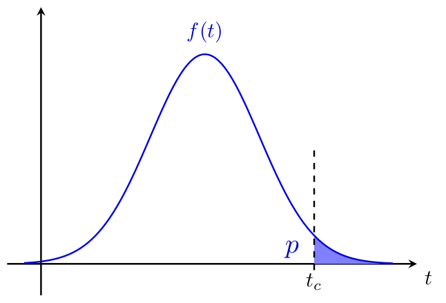
p-value
p-value is defined as the tail probability of a test statistic. While conducting hypothesis tests manually, i.e. with a pencil on paper, use of a p-value is not essential, since calculation of p-value already requires a calculated test statistic. In some cases, we may need to do so, though. A p-value is especially practical when we do our analysis on a computer using a dedicated software. The rule is simple:
\(H_{0}\) is rejected if \(p-value < \alpha\)
A course-related/pedagogical warning about the p-value is that, my expectation (from students) is to see the proper use of ’test score vs critical value’ comparisons in concluding hypothesis tests rather than \(p-value\) vs \(\alpha\)’ comparisons, unless otherwise stated. In your future/professional practice you will have full freedom to enjoy \(p-value\)s.
Type I and Type II errors and the Power of a hypothesis test
Despite Power is not a difficult concept to grasp intuitively, its mathematics is often confusing to students. Patiently go over the following:
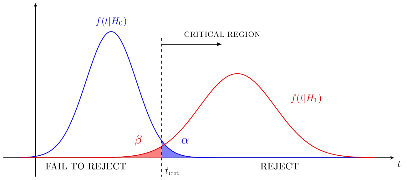
As you may recall, a Type I error occurs if the researcher rejects the null hypothesis in favor of the alternative hypothesis when, in fact, the null hypothesis is true. The probability of Type I error is denoted as \(\alpha\). A Type II error, on the other hand, occurs if the researcher fails to reject the null hypothesis when, in fact, the null hypothesis is false. The probability of Type II error is denoted as \(\beta\). So,
\[\begin{aligned} \operatorname{P}\!\left(\text{Reject } H_{0}\,\middle|\,H_{0}\text{ true}\right) &= \alpha \\ \operatorname{P}\!\left(\text{Fail to reject } H_{0}\,\middle|\,H_{0}\text{ true}\right) &= 1-\alpha \\ \operatorname{P}\!\left(\text{Fail to reject } H_{0}\,\middle|\,H_{0}\text{ false}\right) &= \beta \\ \end{aligned}\]
\[\begin{aligned} \text{Power}=1-\beta & =\operatorname{P}\!\left(\text{Fail to reject } H_{0}\,\middle|\,H_{0}\text{ false}\right)\\ & = \operatorname{P}\!\left(\text{Reject } H_{0}\,\middle|\,H_{0}\text{ false}\right) \end{aligned}\]
So, in plain language, \(Power\) is the ability of a test to avoid a false null hypothesis.
(As a caution, note that there is no requirement of any sort like \(\alpha+\beta=1\))
As you may pick infinitely many alternative values for your parameter of interest, there is a multiplicity of values for Power. So, Power, is indeed a function. We often write it as a function of the difference between the alternative and hypothesized parameter values.
As a closing remark, drawing graphs (rather than calculating) may be very useful to understand the Type II error as well as Power.
Exercise. In a two-sided (two-tailed) hypothesis test, the test statistic was calculated as \(0.18\). We know that the distribution of the test statistic (call this A distribution) has the triangular shaped union of the line segments \([AB]\) and \([BC]\), given \(A(0.00,0.00)\), \(B(2.00,0.50)\) and \(C(4.00,0.00)\). Conclude the test at \(\alpha = 0.005\) by calculating and using p-values only. In your answer, clearly define what p-value is.
Solution. This exercise is left as self-study.
Referring to \(H_{0}: \mu = 0\) against \(H_{1}: \mu>0\) and using proper drawings of the relevant distributions, demonstrate that
Power of a hypothesis test gets higher as the sample size gets larger Power of a hypothesis test gets higher as population variance gets smaller
Make sure your drawings are clear and well-explained.
Solution. This exercise is left as self-study.
Consider a large box which contains many white (\(W\)) and black (\(B\)) balls. We have forgotten the percentage of white balls in the box, but remember that it is either \(\frac{1}{3}\) or \(\frac{2}{3}\). Even though we do not know the percentage of white balls in the box we strongly believe that it is \(\frac{1}{3}\) (but still believe that it might be \(\frac{2}{3}\)). Hence we decide to test if the percentage of white balls in the box is \(\frac{2}{3}\). For this purpose we draw \(20\) balls at random with replacement and note their color.
What are the hypotheses of this test? If we decide to use the number of white balls as our test statistic, what is the distribution of the test statistic? What is the decision rule? If the sample you observed was:
\(W\) \(W\) \(W\) \(B\) \(B\) \(W\) \(B\) \(W\) \(B\) \(W\) \(B\) \(B\) \(W\) \(B\) \(W\) \(B\) \(W\) \(W\) \(W\) \(W\)
what would your conclusion be? What is the p-value corresponding to the above sample? What is the probability of a Type I error and the probability of a Type II error?
Solution. This exercise is left as self-study.
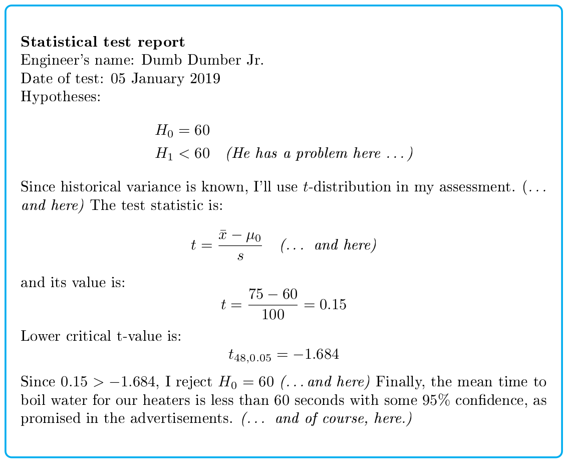
In the investigation of the average performance of produced kettles, a quality control engineer examines \(49\) kettles and measures the mean time to heat \(1\) liter of water from \(25\circ C\) to \(100\circ C\) as \(75 seconds\). Knowing that this had a historical variance of \(100 seconds^{2}\), he wants to test at \(\alpha = 0.05\) whether the population mean time is equal to \(60 seconds\) or not, as the producer’s advertisements say "\(1\) liter in \(1\) minute". Help him to correct the mistakes in his statistical test report.
Solution. The hypotheses involved should be written as: \[\begin{aligned} &H_{0}: \mu=60 \\ &H_{1}: \mu>60 \end{aligned}\] As the historical variance of temperatures is known to be \(100\), the researcher should use: \[z=\frac{75-60}{10}=1.5\] where the upper-critical z-value is \(1.65\) in this one-sided test. Since \(1.5<1.65\), we fail to reject \(H_{0}\). The mean time to boil water is not longer than \(60\) seconds, as promised in the advertisements.
A researcher investigates whether two different teaching methods yield similar impacts on learning of students. After Method \(1\) is used in Section \(1\) and Method \(2\) is used in Section \(2\) of the same course, the same final exam is given to both sections. Then the researcher forms a \(95\%\) confidence interval as \(\left[9.82, 17.30\right]\) for the difference of exam grades (Section \(1\) grade minus Section \(2\) grade). Can you analyze whether there is a difference of \(15 points\) between the grades of two sections?
Solution. This exercise is left as self-study.
The choice of confidence level \(\left(1-\alpha\right)\) for statistical practices depend on the scientific/technical discipline. Referring to an economist/financial analyst (performing portfolio analysis), a computer scientist (designing and coding national payment systems), an international relations specialist (trying to avoid nuclear conflicts) and a physicist working for the CERN (searching for a very rare subatomic particle), explain how the confidence level must be chosen.
Solution. This exercise is left as self-study.
We have the following information:
Researcher A tests \(H_{1}:\sigma^{2} > a\) against \(H_{0}:\sigma^{2} \leq a\) at \(\alpha = 0.05\) and she uses in her report the critical value of \(c_{1}\) to conduct and conclude the test, using a sample of size \(n_{1}\).
Researcher B tests \(H_{1}:\sigma^{2} \neq b\) against \(H_{0}:\sigma^{2} = b\) at \(\alpha = 0.10\) and she uses in her report the critical values of \(d_{1}\) and \(d_{2}\), where \(d_{1} < d_{2}\), to conduct and conclude the test, using a sample of size \(n_{2}\).
Researcher C tries to test \(H_{1}:\sigma_{X}^{2} > \sigma_{Y}^{2}\) against \(H_{0}:\sigma_{X}^{2} \leq \sigma_{Y}^{2}\) at \(\alpha = 0.05\), using \(n_{2}\) observations of \(X\) and \(n_{1}\) observations of \(Y\). Unfortunately, he only has his own data of \(X\) and \(Y\) as well as the research reports of Researcher A and Researcher B, but he does not have a computer or any statistical tables.
Help him to find the critical value needed.
Solution. This exercise is left as self-study.