Chapter 4
Sampling distributions
This chapter bridges our knowledge of the probability theory to statistical inference. Sampling distributions is the key to our understanding of how a small portion of a whole can represent the whole.
Chebyshev’s theorem
For any random variable \(X\) with a finite expected value \(\mu\) and finite variance \(\sigma^2\),
\[\forall k > 1, \operatorname{P}\!\left(|X - \mu| \leq k\sigma\right) \geq 1 - \frac{1}{k^{2}}\]
or, alternatively, by setting \(k = \frac{\epsilon}{\sigma}\),
\[\forall \epsilon > 0, \operatorname{P}\!\left(|X - \mu| \leq \epsilon\right) \geq 1 - \frac{1}{\frac{\epsilon^{2}}{\sigma^{2}}}\]
When \(\sigma^{2}\) is known, one of the \(k\) and \(\epsilon\) can be arbitrarily picked.
Law of large numbers theorem
Let \(\left\{X_{i}\right\}_{i = 1}^{N}\) be a sequence of identically and independently distributed random variables with a finite expected value \(\mu\). For each \(n \leq N\), define the random variable \(\bar{X}_{n}\) as:
\[\bar{X}_{n} = \frac{X_{1} + X_{2} + \cdots + X_{n}}{n}\]
Then,
\[\forall \epsilon > 0, \lim_{n \to \infty}\operatorname{P}\!\left(|\bar{X}_{n} - \mu| \leq \epsilon\right) = 1\]
For sufficiently large \(n\), the mean of independently and identically distrbuted (i.i.d.) \(n\) random variables will almost surely be arbitrarily close to the expected value of the individual random variables.
Noting that, \(\operatorname{E}\!\left(\bar{X}_{n}\right)= \mu\) and \(\operatorname{Var}\left(\bar{X}_{n}\right) = \frac{\sigma^2}{n}\) Then, \(\forall n \leq N, \forall \epsilon > 0\),
\[\operatorname{P}\!\left(|\bar{X}_{n} - \mu| \leq \epsilon\right) \geq 1 - \frac{1}{\frac{\epsilon^{2}}{\sigma^{2}/n}}\]
as implied by the Chebyshev’s theorem. As \(n\) approaches infinity, this expression reduces to:
\[\forall \epsilon > 0, \lim_{n \to \infty} \operatorname{P}\!\left(|\bar{X}_{n} - \mu| \leq \epsilon\right) = 1\]
which is known as the Law of large numbers and is true even when the variance of \(X_i\) is not finite.
Central limit theorem
Let \(\left\{X_{i}\right\}_{i = 1}^{N}\) be a sequence of identically and independently distributed random variables with a finite expected value \(\mu\), and a finite and positive variance \(\sigma^{2}\). For each \(n\), define the random variable \(\bar{X}_{n}\) as:
\[\bar{X}_{n} = \frac{X_{1} + X_{2} + \cdots + X_{n}}{n}\]
Let \(Z\) be a standard normal random variable. For any \(z \in \mathbb{R}\), we have
\[\lim_{n \to \infty} \operatorname{P}\!\left(\frac{\bar{X}_{n} - \mu}{\frac{\sigma}{\sqrt{n}}} \leq z\right) = \operatorname{P}\!\left(Z \leq z\right)\]
Informally, CLT states that for sufficiently large \(n\), the random variable
\[\frac{\bar{X}_{n} - \mu}{\frac{\sigma}{\sqrt{n}}}\]
is approximately standard normal distributed regardless of the distribution of \(X_i\) and exactly standard normal distributed if \(X_i\) are normally distributed.
Distribution of sample means
Consider \(\left\{x_{i}\right\}_{i=1}^{n} \subset \left\{x_{i}\right\}_{i=1}^{N}\) which is a random sample of \(n\) observations coming from a population with mean \(\mu\) and variance \(\sigma^{2}\). \(X_{n}\) being \(\bar{X}_{n} = \frac{X_{1} + X_{2} + \cdots + X_{n}}{n}\) \[\operatorname{E}\!\left(\bar{X}_{n}\right) = \mu\] \[\operatorname{Var}\left(\bar{X}_{n}\right) = \frac{\sigma^2}{n}\] If the population is distributed normally, then the distribution of the sample means is also normal. So, \[Z = \frac{\bar{X}_{n} - \mu}{\frac{\sigma}{\sqrt{n}}}\] has a standard normal distribution.
Essence of sampling distributions
Distribution of sample proportions
Consider \(\left\{x_{i}\right\}_{i=1}^{n} \subset \left\{x_{i}\right\}_{i=1}^{N}\) which is a random sample of \(n\) observations coming from a \(\operatorname{Bernoulli}(p)\) population. \(X_{n}\) being \(\bar{X}_{n} = \frac{X_{1} + X_{2} + \cdots + X_{n}}{n} = \hat{p}\)
\(\operatorname{E}\!\left(\hat{p}\right) = p\)
\(\operatorname{Var}\left(\hat{p}\right) = \frac{p\left(1-p\right)}{n}\)
If \(n\) is large, \[Z = \frac{\hat{p} - p}{\sqrt{\frac{p\left(1-p\right)}{n}}}\] is approximately distributed as a standard normal.
Distribution of sample variances
Let \(s^2\) denote the sample variance for a random sample of \(n\) observations from a population with a variance of \(\sigma^{2}\).
\(\operatorname{E}\!\left(s^{2}\right) = \sigma^2\)
\(\operatorname{Var}\left(s^{2}\right) = \frac{2\sigma^4}{n-1}\)
\[\begin{aligned} \sum_{i=1}^{n}(x_{i}-\bar{x})^{2}= & \sum((x_{i}-\mu)-(\bar{x}-\mu))^{2} \\ = & \sum(x_{i}-\mu)^{2}-2(\bar{x}-\mu)\sum(x_{i}-\mu)+\sum(\bar{x}-\mu)^{2} \\ = & \sum(x_{i}-\mu)^{2}-2n(\bar{x}-\mu)^{2}+n(\bar{x}-\mu)^{2} \\ = & \sum(x_{i}-\mu)^{2}-n(\bar{x}-\mu)^{2} \\ \end{aligned}\]
\[\begin{aligned} \operatorname{E}\!\left(\sum(x_{i}-\bar{x})^{2}\right)= & \operatorname{E}\!\left(\sum(x_{i}-\mu)^{2}\right)-n \operatorname{E}\!\left((\bar{x}-\mu)^{2}\right) \\ = & \sum \underbrace{\operatorname{E}\!\left((x_i-\mu)^2\right)}_{\sigma^2}-n \underbrace{\operatorname{E}\!\left((\bar{x}-\mu)^{2}\right)}_{\sigma^2/n} \\ = & n \sigma^{2}-n \frac{\sigma^{2}}{n}=(n-1) \sigma^{2} \end{aligned}\]
So,
\[\begin{aligned} \operatorname{E}\!\left(s^{2}\right)= & \operatorname{E}\!\left(\frac{1}{n-1}\sum(x_{i}-\bar{x})^{2}\right) \\ = & \frac{1}{n-1}\operatorname{E}\!\left(\sum(x_{i}-\bar{x})^{2}\right) \\ = & \frac{1}{n-1}(n-1)\sigma^{2}=\sigma^{2} \end{aligned}\]
Given a random sample of \(n\) observations from a normally distributed population whose variance is \(\sigma^{2}\), the sample variance \(s^2\) has a \(\chi^2\) distribution with \((n-1)\) degrees of freedom? \[\chi^2_{n-1} = \frac{\left(n-1\right) s^{2}}{\sigma^{2}}\] is distributed as the Chi-squared \(\left(\chi^{2}\right)\) distribution with \(\left(n-1\right)\) degrees of freedom.
Exercise. We have two data sets consisting of identical values: \(0\), \(1\), \(2\), \(3\), \(4\), \(5\), \(6\), \(7\), \(8\), \(9\), \(10\). We will use \(x_i\) denote the \(i^{th}\) value in one data set and \(y_{j}\) to denote the \(j_{th}\) value in the other data set. We construct a new data set by taking a number from each data set and finding their average, i.e.. the new data set consists of values of the form: \[\frac{\left(x_{i} + y_{j}\right)}{2}\] The constructed data set will consist of one \(0\), two \(0.5\)’s, three \(1\)’s, etc.
Find all values in the new data set and their corresponding frequencies Construct a graph that summarize your finding Find the mean and variance of the initial data set and the new data set
Solution. Solve yourself to explore the Central Limit Theorem.
We make \(100\) independent observations from a population with mean \(40\) and standard deviation \(20\). Approximately, what is the probability that the mean of these observations will be greater than \(37\)?
Solution. Population \(X \sim \cdot(40,20^2)\). We take \(n=100\) observations and calculate \(\bar{X}_{100}\). \[\begin{aligned} \operatorname{E}\!\left(\bar{X}_{100}\right) & =\mu=40 \\ \operatorname{Var}\left(\bar{X}_{100}\right) & =\frac{\sigma^{2}}{n}=\frac{400}{100}=4 \\ \operatorname{P}\!\left(\bar{X}_{100}>37\right) & =\operatorname{P}\!\left(\frac{\bar{X}_{100}-40}{\sqrt{4}}>\frac{37-40}{\sqrt{4}}\right) \\ & =\operatorname{P}\!\left(z>-1.5\right) \\ & =0.93319 \end{aligned}\]
The following table gives the relative frequency distribution of a population:
Value Rel. Freq. \(2\) \(0.1\) \(4\) \(0.3\) \(6\) \(0.2\) \(8\) \(0.3\) \(10\) \(0.1\) A number is selected from this population at random, what is the probability that the number selected is greater than or equal to \(8\)? If we select two numbers at random (with replacement), what is the probability that the mean of these two numbers is less than or equal to \(5\)? If \(25\) numbers are selected from the population at random (with replacement), what is the probability (approximately) that the mean these \(25\) numbers is less than \(6.5\)?
Solution.
The only trick in this exercise is to begin with calculating \(\operatorname{E}\!\left(X\right)\) and \(\operatorname{Var}\left(X\right)\). Calculate and see \(\operatorname{E}\!\left(X\right)=6\) and \(\operatorname{Var}\left(X\right)=5.6\). There is no sampling as \(n=1\). Simply calculate \(\operatorname{P}\!\left(X \geq 8\right)\).
Calculate \(\operatorname{P}\!\left(\bar{X}_{2} \leq 5\right)\).
Calculate \(\operatorname{P}\!\left(\bar{X}_{25}<6.5\right)\). Remember that \(\operatorname{E}\!\left(\bar{X}_{n}\right)=\mu\) and \(\operatorname{Var}\left(\bar{X}_{n}\right)=\sigma^{2} / n\).
We choose \(36\) numbers, with replacement, at random (i.e.., we take a random sample of size \(36\)) from the interval \(\left(0,4\right)\). Let \(X\) be the random variable that assigns to each sample (outcome) the mean of the sample.
Find the expected value and variance of \(X\) Find (an approximate value for) the probability that the sample mean, i.e.. \(X\), will be less than or equal to \(2.3\)
Solution.
Since nothing further is instructed, assume that the population is \(\operatorname{Uniform}(0,4)\). Then, \[\begin{aligned} \mu & =\frac{0+4}{2}=2 \\ \sigma^{2} & =\frac{(4-0)^{2}}{12}=\frac{16}{12} \end{aligned}\] \(X\), here, is the mean of our 36 observations, i.e., \(\bar{X}_{36}\) in our usual notation. \[\begin{aligned} \operatorname{E}\!\left(X\right) & =\mu=2 \\ \operatorname{Var}\left(X\right) & =\frac{\sigma^{2}}{n}=\frac{16 / 12}{36}=\frac{1}{27} \end{aligned}\]
Using the parameters in part (i), calculate \(\operatorname{P}\!\left(X \leq 2.3\right)\), i.e., \(\operatorname{P}\!\left(z \leq 1.56\right)\). The answer is \(0.94062\).
We choose \(9\) numbers from a normally distributed population of numbers. The mean of the population is unknown but the variance is know to be equal to \(16\). If \(\mu\) denotes the mean of the population, then what is the probability that the mean of the \(9\) numbers that we choose will be in the interval \(\left[\mu-2, \mu+2\right]\)?
Solution. You do not need the value of \(\mu\) in this exercise. The key to solution is that \(\operatorname{Var}\left(\bar{X}_{9}\right)=16 / 9\). So, performing the intermediate steps, the problem reduces to finding \(\operatorname{P}\!\left(-1.5 \leq z \leq 1.5\right)\) and the answer is \(0.86638\).
In a certain university the CGPA’s of students only takes the values \(0\), \(1\), \(2\), \(3\), \(4\). The distribution of CGPA’s of students of this university is given below:
CGPA Freq \(0\) \(5,000\) \(1\) \(10,000\) \(2\) \(20,000\) \(3\) \(5,000\) \(4\) \(10,000\) Total \(50,000\) Let \(\bar{X}_{1}\) denote the CGPA of a student who was chosen at random from the population of all students of this university. Tabulate the PDF of this random variable. Let \(\bar{X}_{2}\) denote the average (mean) of the CGPA’s of two randomly selected students from the population of all students of this university. What is the probability that the average CGPA of the two students is less than or equal to \(1\)? Now we choose \(36\) students at random. What is the probability, approximately, that the average CGPA of these students (\(\bar{X}_{36}\)) is less than or equal to \(2.3\)?
Solution. This exercise is left as self-study.
Consider a large population of which only \(20\%\) know basic concepts of statistics. We take a random sample of size \(81\) from this population and count the number of individuals, in the sample, who knows basic concepts of statistics. What is the probability that the sample will have between \(15\) and \(18\) (inclusive) individuals who know basic concepts of statistics?
Solution. This exercise is left as self-study.
A four sided fair die is rolled several times and we calculate the average (mean) of the values observed.
Let \(X_1\) denote the random variable that gives the value observed when the die is rolled once. Find the expected value and variance of \(X_1\). Let \(\bar{X}_{n}\) denote the mean of the values observed when the die is rolled \(n\) times. What is the minimum number of times that the die should be rolled so that the mean (the value of \(\bar{X}_{n}\)) takes a value in the interval \(\left[2.1,2.9 \right]\) with at least a probability of \(0.9\)? Use \(Chebyshev's Theorem\) to answer this problem. Using the \(Central Limit Theorem\) and the value for \(n\) you found above, find an approximate value for the probability of \(\bar{X}_{n}\) taking a value in the interval \(\left[2.1,2.9\right]\). Do the answers you found in item \(\left(ii\right)\) and item \(\left(iii\right)\) contradict each other? If there is a difference in what the two answers suggest, explain the reason for this.
Solution. i. When the die is rolled once, by definition we produce an outcome directly of the population (that is we don’t do any sampling at all). So, \[\begin{aligned} X_{1} \sim f\!\left(x\right), f\!\left(x\right)=1 / 4, x=1,2,3,4 \quad \text{(Discrete}RV\text{)} \\ \end{aligned}\]
\[\begin{aligned} \operatorname{E}\!\left(X_{1}\right) & =1\cdot1/4+2\cdot1/4+3\cdot1/4+4\cdot1/4 \\ & =2.5 \end{aligned}\]
\[\begin{aligned} \operatorname{E}\!\left(X_{1}^{2}\right) & =1\cdot1/4+4\cdot1/4+9\cdot1/4+16\cdot1/4 \\ & =7.5 \end{aligned}\]
\[\begin{aligned} \operatorname{Var}\left(X_{1}\right) & =7.5-2.5^{2} \\ & =1.25 \end{aligned}\]
So, \(X_{1}\sim\cdot(2.5,1.25)\)
ii. \(\bar{X}_{n}\) is the RV denoting the sample mean, when We roll the die \(n\) times. \[\begin{array}{l} \operatorname{E}\!\left(\bar{X}_{n}\right)=\operatorname{E}\!\left(X_{1}\right)=2.5 \\ \operatorname{Var}\left(\bar{X}_{n}\right)=\frac{\operatorname{Var}\left(X_{1}\right)}{n}=\frac{1.25}{n} \end{array}\]
Midpoint of the interval \([2.1,2.9]\) is \(2.5\)
\[\begin{gathered} \operatorname{E}\!\left(X_{1}\right)=\operatorname{E}\!\left(\bar{X}_{n}\right)=2.5 \\ 2.5-2.1=2.9-2.5=0.4 \rightarrow \epsilon\\ \epsilon=0.4 \end{gathered}\] \[\begin{aligned} \operatorname{P}\!\left(|\bar{X}_{n}-2.5|\leq0.4\right)\geq & 1-\frac{1}{\frac{0.4^{2}}{\frac{1.25}{n}}} \leftarrow 0.9 \\ \end{aligned}\] \[\begin{aligned} & 1-\frac{1}{\frac{0.4^{2}}{\frac{1.25}{n}}}=0.9 \\ & \frac{1.25}{n}=0.1\times 0.16 \\ \end{aligned}\] \[\begin{aligned} n & =\frac{1.25}{0.016} \\ & =78.125 \\ n & =79 \leftarrow \text{Round 78.125 up} \end{aligned}\] Notice that in this part, we use the Chebyshev’s theorem only. We get: \[\begin{aligned} & \operatorname{E}\!\left(\bar{X}_{79}\right)=2.5 \\ \end{aligned}\] and \[\begin{aligned} & \operatorname{Var}\left(\bar{X}_{79}\right)=\frac{1.25}{79}=0.015823 \\ \end{aligned}\]
iii. \[\begin{aligned} \operatorname{P}\!\left(2.1 \leq \bar{X}_{79} \leq 2.9\right) & =\operatorname{P}\!\left(\frac{2.1-2.5}{\sqrt{0.015823}} \leq z \leq \frac{2.9-2.5}{\sqrt{0.015823}}\right) \\ & =\operatorname{P}\!\left(\frac{-0.4}{0.1258} \leq z \leq \frac{0.4}{0.1258}\right) \\ & =0.99852 \end{aligned}\] Notice that in this part, we use the CLT only.
iv. No, they don’t contradict each other: While Chebyshev’s theorem sets a lowerbound of 0.90 here (in ii), (iii) gives the actual probability as 0.99852 which is larger than 0.90 (as it should be).
Though I am not a fan of such hints, here a useful hint may be underlined: When an interval is given in a question like this, always begin with observing (calculating) its midpoint. In this question, the midpoint was \((2.1+2.9) / 2=2.5\), which is nothing but \(\operatorname{E}\!\left(X_{1}\right)\) and \(\operatorname{E}\!\left(\bar{X}_{n}\right)\). Once you have noticed this, it will be trivial to find \(\epsilon\) to figure out the rest of the steps.
One additional point is: \[\bar{X}_{1}=\frac{X_{1}}{1}\]
So, sampling with \(n=1\) simply refers to population’s distribution.
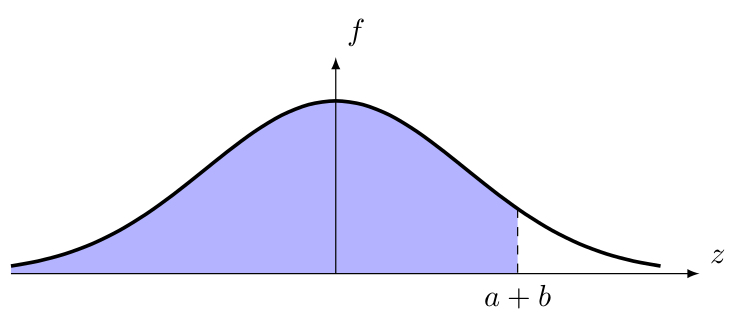
Ztandard Normal Diztribution
A cell which is at the intersection of the row labeled with \(a\) and column labeled with \(b\) gives the probability \(\operatorname{P}\!\left(Z \leq a+b\right)\).
| \(z\) | 0.00 | 0.01 | 0.02 | 0.03 | 0.04 | 0.05 | 0.06 | 0.07 | 0.08 | 0.09 |
|---|---|---|---|---|---|---|---|---|---|---|
| 0.00 | 0.5000 | 0.5040 | 0.5080 | 0.5120 | 0.5160 | 0.5199 | 0.5239 | 0.5279 | 0.5319 | 0.5359 |
| 0.10 | 0.5398 | 0.5438 | 0.5478 | 0.5517 | 0.5557 | 0.5596 | 0.5636 | 0.5675 | 0.5714 | 0.5754 |
| 0.20 | 0.5793 | 0.5832 | 0.5871 | 0.5909 | 0.5948 | 0.5987 | 0.6026 | 0.6064 | 0.6103 | 0.6141 |
| 0.30 | 0.6179 | 0.6217 | 0.6255 | 0.6293 | 0.6331 | 0.6368 | 0.6406 | 0.6443 | 0.6480 | 0.6517 |
| 0.40 | 0.6554 | 0.6591 | 0.6628 | 0.6664 | 0.6700 | 0.6736 | 0.6772 | 0.6808 | 0.6844 | 0.6879 |
| 0.50 | 0.6915 | 0.6950 | 0.6985 | 0.7019 | 0.7054 | 0.7088 | 0.7123 | 0.7157 | 0.7190 | 0.7224 |
|---|---|---|---|---|---|---|---|---|---|---|
| 0.60 | 0.7258 | 0.7291 | 0.7324 | 0.7357 | 0.7389 | 0.7421 | 0.7454 | 0.7486 | 0.7518 | 0.7549 |
| 0.70 | 0.7580 | 0.7611 | 0.7642 | 0.7673 | 0.7703 | 0.7734 | 0.7764 | 0.7793 | 0.7823 | 0.7852 |
| 0.80 | 0.7881 | 0.7910 | 0.7939 | 0.7967 | 0.7995 | 0.8023 | 0.8051 | 0.8078 | 0.8106 | 0.8133 |
| 0.90 | 0.8159 | 0.8186 | 0.8212 | 0.8238 | 0.8264 | 0.8289 | 0.8315 | 0.8340 | 0.8365 | 0.8389 |
| 1.00 | 0.8413 | 0.8438 | 0.8461 | 0.8485 | 0.8508 | 0.8531 | 0.8554 | 0.8577 | 0.8599 | 0.8621 |
|---|---|---|---|---|---|---|---|---|---|---|
| 1.10 | 0.8643 | 0.8665 | 0.8686 | 0.8708 | 0.8729 | 0.8749 | 0.8770 | 0.8790 | 0.8810 | 0.8830 |
| 1.20 | 0.8849 | 0.8869 | 0.8888 | 0.8906 | 0.8925 | 0.8943 | 0.8962 | 0.8980 | 0.8997 | 0.9015 |
| 1.30 | 0.9032 | 0.9049 | 0.9066 | 0.9082 | 0.9099 | 0.9115 | 0.9131 | 0.9147 | 0.9162 | 0.9177 |
| 1.40 | 0.9192 | 0.9207 | 0.9222 | 0.9236 | 0.9251 | 0.9265 | 0.9279 | 0.9292 | 0.9306 | 0.9319 |
| 1.50 | 0.9332 | 0.9345 | 0.9357 | 0.9370 | 0.9382 | 0.9394 | 0.9406 | 0.9418 | 0.9429 | 0.9441 |
|---|---|---|---|---|---|---|---|---|---|---|
| 1.60 | 0.9452 | 0.9463 | 0.9474 | 0.9484 | 0.9495 | 0.9505 | 0.9515 | 0.9525 | 0.9535 | 0.9545 |
| 1.70 | 0.9554 | 0.9564 | 0.9573 | 0.9582 | 0.9591 | 0.9599 | 0.9608 | 0.9616 | 0.9625 | 0.9633 |
| 1.80 | 0.9641 | 0.9649 | 0.9656 | 0.9664 | 0.9671 | 0.9678 | 0.9686 | 0.9693 | 0.9699 | 0.9706 |
| 1.90 | 0.9713 | 0.9719 | 0.9726 | 0.9732 | 0.9738 | 0.9744 | 0.9750 | 0.9756 | 0.9761 | 0.9767 |
| 2.00 | 0.9772 | 0.9778 | 0.9783 | 0.9788 | 0.9793 | 0.9798 | 0.9803 | 0.9808 | 0.9812 | 0.9817 |
|---|---|---|---|---|---|---|---|---|---|---|
| 2.10 | 0.9821 | 0.9826 | 0.9830 | 0.9834 | 0.9838 | 0.9842 | 0.9846 | 0.9850 | 0.9854 | 0.9857 |
| 2.20 | 0.9861 | 0.9864 | 0.9868 | 0.9871 | 0.9875 | 0.9878 | 0.9881 | 0.9884 | 0.9887 | 0.9890 |
| 2.30 | 0.9893 | 0.9896 | 0.9898 | 0.9901 | 0.9904 | 0.9906 | 0.9909 | 0.9911 | 0.9913 | 0.9916 |
| 2.40 | 0.9918 | 0.9920 | 0.9922 | 0.9925 | 0.9927 | 0.9929 | 0.9931 | 0.9932 | 0.9934 | 0.9936 |
| 2.50 | 0.9938 | 0.9940 | 0.9941 | 0.9943 | 0.9945 | 0.9946 | 0.9948 | 0.9949 | 0.9951 | 0.9952 |
|---|---|---|---|---|---|---|---|---|---|---|
| 2.60 | 0.9953 | 0.9955 | 0.9956 | 0.9957 | 0.9959 | 0.9960 | 0.9961 | 0.9962 | 0.9963 | 0.9964 |
| 2.70 | 0.9965 | 0.9966 | 0.9967 | 0.9968 | 0.9969 | 0.9970 | 0.9971 | 0.9972 | 0.9973 | 0.9974 |
| 2.80 | 0.9974 | 0.9975 | 0.9976 | 0.9977 | 0.9977 | 0.9978 | 0.9979 | 0.9979 | 0.9980 | 0.9981 |
| 2.90 | 0.9981 | 0.9982 | 0.9982 | 0.9983 | 0.9984 | 0.9984 | 0.9985 | 0.9985 | 0.9986 | 0.9986 |
| 3.00 | 0.9987 | 0.9987 | 0.9987 | 0.9988 | 0.9988 | 0.9989 | 0.9989 | 0.9989 | 0.9990 | 0.9990 |
|---|---|---|---|---|---|---|---|---|---|---|
| 3.10 | 0.9990 | 0.9991 | 0.9991 | 0.9991 | 0.9992 | 0.9992 | 0.9992 | 0.9992 | 0.9993 | 0.9993 |
| 3.20 | 0.9993 | 0.9993 | 0.9994 | 0.9994 | 0.9994 | 0.9994 | 0.9994 | 0.9995 | 0.9995 | 0.9995 |
| 3.30 | 0.9995 | 0.9995 | 0.9995 | 0.9996 | 0.9996 | 0.9996 | 0.9996 | 0.9996 | 0.9996 | 0.9997 |
| 3.40 | 0.9997 | 0.9997 | 0.9997 | 0.9997 | 0.9997 | 0.9997 | 0.9997 | 0.9997 | 0.9997 | 0.9998 |