Chapter 8
Linear regression analysis
In the previous chapters that served the whole ECON 221 and about a half of ECON 222, we studied the fundamentals of Probability theory and the key theory and toolset of Statistical inference. Remember that we focused solely on understanding statistical distributions and estimating the distributional parameters. In your future scientific, technical, professional practice, this body of knowledge will be quite fruitful.
Now, we are ready to study the theoretical background and applied dimensions of the ’curve-fitting’ problem. To this end, in this chapter, we will consider the Linear Regression Models. Notice that what we will do here accounts for the first half of a traditionally designed ’Introductory Econometrics’ course.
The term regression was coined by Francis Galton to describe a biological phenomenon. The phenomenon was that the heights of descendants of tall ancestors tend to regress down towards a normal average, which is also known as regression toward the mean. For Galton, regression had only this biological meaning. His work was later extended by Udny Yule and Karl Pearson, and later by Fisher (in a way to come closer to Gauss’s 1821 formulation of the problem). Once you have researched it, you will enjoy the history of this certain line of research.
As being the main pillar of it, the ’regression analysis’ takes us to the rich analytical world of Econometrics. The literal meaning of the term econometrics (econo\(+\)metrics) is ’measurement in economics’. Econometrics is ’the branch of economics concerned with the use of statistical methods in describing and quantifying economic systems’ (Oxford Dictionary). From a broader perspective, econometrics is a shared sub-field of Statistics (hence of Mathematics) and Economics. In that, our tools in Econometrics are those tools in Statistics as shaped and augmented by our knowledge of Economics. (One of the founders of the Econometrics Society, another pioneer of the field, Ragnar Frisch is credited with coining the term ’econometrics’.)
Renowned academic Badi Baltagi says “An econometrician has to be a competent mathematician and statistician who is an economist by training. Fundamental knowledge of mathematics, statistics and economic theory are a necessary prerequisite for this field”.
Our starting point is a scientific urge to find/formulate, measure and test the relationship between, say, two variables \(y\) and \(x\). These variables may belong to natural sciences, social sciences or even to humanities; this is not something to mind. What matters often is that the linkage between our variables may not be (mostly is not) a perfect relationship like \(y=mx+n\) (we prefer indeed a notation like \(y=\beta_0+\beta_1x\), where \(n\) is \(\beta_0\) and \(m\) is \(\beta_1\)). We rather observe there are deviations from a perfect relationship, as seen earlier in ECON 221. In that, actual \(y\) values are connected to actual \(x\) values through a relationship like \(y=\beta_0+\beta_1x+e\) where \(e\) stands for a sequence of statistical errors (disturbances).
The error sequence \(e\) may stem from the random actions/choices of humans, unexpected shocks to socio-economic systems, misspecification of models, improper choices of mathematical functional forms or imprecision of the data. Note that, this picture is not specific to social sciences: in the natural science experiments there is a multiplicity of sources of uncertainty (hence of statistical errors or disturbances).
Goals of econometrics, as we understand it, will be (1) to find the relation between variables \(y\) and \(x\), encapsulated in \((\beta_0,\beta_1)\), (2) to validate and quantify theory and (3) forecasting.
Purpose of modeling and Simplicity
Deferring a detailed discussion of it to class gatherings, we will say here that ’a model is a downsized yet realistic representation of reality’. An immediate analogy from architecture would be useful: on an architectural model of a building we see things ’only as needed’. While we may not see the doorknobs (depending on the scale) on a model, we see the proportionality of distances clearly. After all, the purpose of the model is to give a broad yet accurate idea of/about things.
A similar idea applies in the other disciplines. In business models we do not see every tiny detail of the workplace or the manufacturing environment. In economic models we tend not to include all potential explanatory variables at once. We just try to remain ’accurate enough’.
Using our models we can present our scientific grasp of the nature or universe or the society. Once the model is well-parametrized and quantified, we can develop forecasts of the future, or we can (depending on the type of our model) develop counter factual and/or scenario analyses. Presenting a scientific view of ours and forecasting the future (while) are fairly pragmatic ends, a third use of a scientific model helps testing, validating/ invalidating theories, which calls for a more than pragmatic spirit. Regardless of the purposes cited, though, a model (any model) should display: a certain level of simplicity. Before proceeding, recall Albert Einstein saying "Everything should be made as simple as possible, but no simpler."
In our practice of statistical/ econometric modeling, the ’principle of parsimony’ guides us. Equipped with a rich toolset of formal statistical tests and her judgmental skills, a good researcher tries to come up with an "as simple as possible but no simpler" model. Common sense says essentials will be included in while all the inessentials will be omitted from a model. Bad news is every researcher’s practice has a couple bumps as to improving a sense of such in practice. Good news is honest and hard work pays back.
In Philosophy (and Science) there are several ’razors’ to shave away the redundancies in models (or in scientific explanations). Here we will maintain the Occam’s razor (or Ockham’s razor) attributed to william of Ockham, an English philosopher of the 13th-14th centuries. Occam’s razor is a principle of parsimony stating that among the explanations addressing the same thing, the simplest is to be picked! (William of Baskerville of the Name of the Rose by Umberto Eco is a tribute to William of Ockham) (Arthur Conan Doyle’s Sherlock Holmes once utters "When you have eliminated the impossible, whatever remains, however improbable, must be the truth")
Occam’s razor reads in Latin as "pluralitas non est ponenda sine necessitate" which translates into English as "plurality should not be posited without necessity". The principle, so, calls for parsimony in ’deductive thinking’.
Despite what we do in applied statistics/econometrics is not purely (maybe not at all) deductive thinking, we rather try to reach an inference to the best explanation via a formal sequence of estimations/tests/calculations. In this practice, Occam’s razor sheds some good light for us to see things clearly.
In the world of project development you may hear the same principle as an acronym of ’KISS’. Referring to a model, KISS reads as ’Keep It Small and Simple’ or sometimes as ’Keep It Simple, Stupid’. (Search yourself for its relevance to the US Navy)
In the remainder of this chapter, we will study/learn the theory of elementary econometrics, a rich enough toolset pertaining to it along with a selection of applied problems.
Exercise. Refer to our in-class discussions to explain/discuss the following:
Occam’s razor Principle of parsimony ’Keep It Small and Simple’, i.e., KISS Purpose of modeling Come up with a synthesis of the terms/phrases referred to above.
Solution. Left as self-exercise.
Overview of linear models
Overview of linear models
The specific meaning of linearity here is ’the linearity of a model in terms of (with respect to) its parameters. In that:
\[y=\beta_{0}+\beta_{1} x_{1}+\beta_{2} x_{2}+e\]
is a linear model. So is
\[y=\beta_{0}+\beta_{1} x_{1}^{2}+\beta_{2} x_{2}^{3}+e\]
However,
\[y=\beta_{0}+\beta_{1}^{2} x_{1}+\beta_{1}\beta_{3} x_{2}+\beta_{3}x_{3}+e\]
is not considered to be a linear model. Neither is
\[y=\beta_{0}+\beta_{1} x_{1}+\beta_{2} x_{2}+\beta_{1} \beta_{2} x_{3}+e .\]
In your future practice, you will be able to settle this issue in a crystal clear fashion.
Why do we resort to linear models? This is a very legitimate question once we observe a number of relationships in the nature and in societal life are, indeed, nonlinear (not linear). A straightfor ward answer reads as ’linear models are easy to use’. So, simplicity matters. Simplicity brings practicality to researchers, they are easy to compute, to interpret and to communicate. More importantly, as noted earlier, our linear regression models are linear with respect to their parameters while the independent variables of our models can be of any nonlinear form. All in all, one can establish/ form models that are nonlinear in their variables’ using ’models that are linear in their parameters’. The good thing about models that are linear in parameters is that such a structure allows us to use the tools of linear algebra effectively in our computations.
Our curious nature often forces us to include many explanatory variables in a model: \[y=\beta_{0}+\beta_{1} x_{1}+\beta_{2} x_{2}+\cdots+\beta_{k} x_{k}\]
However, a minimalist design is also possible: \[y=\beta_{0}+\beta_{1} x\]
Even this may be a good enough model (think when): \[y=\beta_{0}\]
The process of inference begins with the specification of an economic model. Then a statistical model describes the sampling process that we visualize was used to produce the sample data. See the structure below:
Economic model: \[y=\beta_{0}+\beta_{1} x\]
Statistical model: \[y=\beta_{0}+\beta_{1} x+e\]
The random error term (\(e\)) serves three main purposes:
\(e\) captures the combined effect of all other influences other than \(x\). These other effects are assumed to be unobservable, otherwise they would be included in the model.
\(e\) captures any approximation error that arises because of the linear functional form
\(e\) captures any element of random behavior present in each individual observation.
See the structures below:
Case 1: Unconditional model of mean
Economic model: \[y=\beta_{0}\]
Statistical model: \[y=\beta_{0}+e\]
Case 2: Simple Linear model
Economic model: \[y=\beta_{0}+\beta_{1} x\]
Statistical model: \[y=\beta_{0}+\beta_{1} x+e\]
Case 3: Multiple Linear model
Economic model: \[y=\beta_{0}+\beta_{1} x_{1}+\beta_{2} x_{2}+\cdots+\beta_{k} x_{k}\]
Statistical model: \[y=\beta_{0}+\beta_{1} x_{1}+\beta_{2} x_{2}+\cdots+\beta_{k} x_{k}+e\]
Transformations and functional forms
Transformations and functional forms In economics and finance, like in other quantitative disciplines, we attribute a great deal of importance to measuring the impact of a change in one variable on one another. Considering \(y=f(x)\) as a relationship between the variables \(y\) (dependent) and \(x\) (independent), the derivative \(d y / d x=f^{\prime}(x)\) describes that impact. When we consider \(y=f\left(x_{1}, x_{2}, \ldots, x_{k}\right)\), the impact of an independent variable \(x_{i}\) on the dependent variable \(y\) is better described by the partial derivative \(\partial y / \partial x_{i}\). Having formed and estimated a proper statistical/ econometric model, then, a researcher gains a good grasp of issues embedded in the research problem at hand.
Note that, as economists and finance specialists, we like to learn about a special class of impact measurements, namely the elasticities. Recall from your introductory economics classes that ’elasticity of \(y\) with respect to \(x\) is the percentage change in \(y\) against a one percentage point change in \(x\) ’. in formal terms:
\[n_{y, x}=\frac{\% \Delta y}{\% \Delta x}=\frac{\frac{\Delta y}{y}}{\frac{\Delta x}{x}}=\frac{\Delta y}{\Delta x} \cdot \frac{x}{y}\]
So, as long as we can estimate \(\Delta y / \Delta x\), we can come up with an estimate of \(\eta_{y, x}\) by substituting appropriate values of \(x\) and \(y\) into \(x / y\). We will see several examples as we progress through this chapter, where we will see estimating an elasticity is possible under a wide array of functional forms of \(f(\cdot)\) in the expression \(y=f(x)\).
One of the functional forms, i.e., the Log-Log form, yields elasticities directly as:
\[\eta_{y, x}=\frac{\Delta \ln y}{\Delta \ln x} .\]
We will discuss this topic further in our classes.
Our approach to teaching/learning
In the remainder of this chapter, we will maintain an approach which may slightly differ from the approaches of others. Sticking to this approach would facilitate better learning. Our approach folds out as:
Depiction of an unconditional model of mean and the mechanics of estimation (without inference)
Depiction of a Simple Linear Regression model and the mechanics of estimation (without inference)
Depiction of a Multiple Linear Regression model and the mechanics of estimation (without inference)
Goodness of fit of a model measured via \(R^{2}\)
Handling statistical uncertainty: calculation of variances and covariances associated with a Multiple Linear Regression model
Statistical inference
Having a pitstop here, the sequence of topics above will provide us with a solid understanding of the mechanical workings of our linear regression universe.
Once we have learned these, we will move to:
Ideal econometric conditions: Gauss-Markov assumptions
In many, maybe all, books Gauss-Markov assumptions are covered before other things. Though, our approach maintains a different pedagogical perspective. In that, we take into consideration the Gauss-Markov assumptions, which are crucial in econometric theory and practice, upon a clear view of the working environment. After that we will move to:
Model specification
Regression analysis at work
Note that the above order of topics require us to stick to it without interruption or gaps for successful learning.
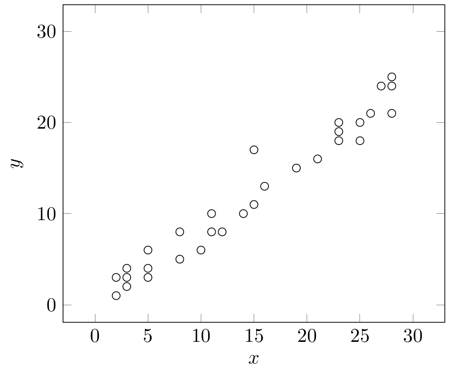
An artificial data set:
In our subsequent discussions we will be referring to the following data set frequently. While we can show a data set as an actual set (with proper mathematical notation) like:
\[\begin{array}{cccccc} \text{A=\{}(2,1),&(2,3),&(3,2),&(3,3),&(3,4),&(5,3),\\ (5,4),&(5,6),&(8,5),&(8,8),&(10,6),&(11,8),\\ (11,10),&(12,8),&(14,10),&(15,11),&(15,17),&(16,13),\\ (19,15),&(21,16),&(23,18),&(23,19),&(23,20),&(25,18),\\ (25,20),&(26,21),&(27,24),&(28,21),&(28,24),&(28,25)\text{\}} \end{array}\]
it may be more practical to use a tabular listing of the data. A tabular structure improves visibility and exposition:
| Observation \(i\) | \(\quad x_i \quad\) | \(\quad y_i \quad\) | Observation \(i\) | \(\quad x_i \quad\) | \(\quad y_i \quad\) |
|---|---|---|---|---|---|
| \(1\) | \(2\) | \(1\) | \(16\) | \(15\) | \(11\) |
| \(2\) | \(2\) | \(3\) | \(17\) | \(15\) | \(17\) |
| \(3\) | \(3\) | \(2\) | \(18\) | \(16\) | \(13\) |
| \(4\) | \(3\) | \(3\) | \(19\) | \(19\) | \(15\) |
| \(5\) | \(3\) | \(4\) | \(20\) | \(21\) | \(16\) |
| \(6\) | \(5\) | \(3\) | \(21\) | \(23\) | \(18\) |
| \(7\) | \(5\) | \(4\) | \(22\) | \(23\) | \(19\) |
| \(8\) | \(5\) | \(6\) | \(23\) | \(23\) | \(20\) |
| \(9\) | \(8\) | \(5\) | \(24\) | \(25\) | \(18\) |
| \(10\) | \(8\) | \(8\) | \(25\) | \(25\) | \(20\) |
| \(11\) | \(10\) | \(6\) | \(26\) | \(26\) | \(21\) |
| \(12\) | \(11\) | \(8\) | \(27\) | \(27\) | \(24\) |
| \(13\) | \(11\) | \(10\) | \(28\) | \(28\) | \(21\) |
| \(14\) | \(12\) | \(8\) | \(29\) | \(28\) | \(24\) |
| \(15\) | \(14\) | \(10\) | \(30\) | \(28\) | \(25\) |
Building and estimating an Unconditional Model of Mean: A model which is a non-model
Consider a variable \(y\) that is modeled as:
\[y=\beta_{0}+e\]
If we have a sample \(y_{1}, y_{2}, \ldots, y_{n}\), this relationship can also be written as
\[y_{i}=\beta_{0}+e_{i}, i=1,2, \ldots, n\]
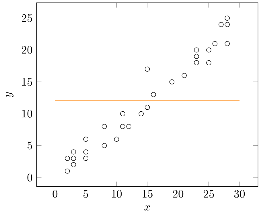
It is clear that our model does not include any independent (explanatory) variables on the right hand side, ie., values of \(y\) are scattered around \(\beta_{0}\) (if they are not all accidentally equal to \(\beta_{0}\) ).
Supposing there are \(K\) potential independent variables, \(x_{1}, x_{2}, \ldots, x_{k}\), that might explain \(y\), the unconditional model of mean can be viewed as:
\[y_{i}=\beta_{0}+0 \cdot x_{1 i}+0 \cdot x_{2 i}+\cdots+0 \cdot x_{k i}+e_{i}\]
where the researcher places zero weight on \(x_{1}, x_{2}, \ldots, x_{k}\). In that, this model of mean turns out to be the simplest possible model or more like a non-model. When we plot \(y_{i}\) against one of the \(x\)’s (say \(x_{ki}\)), the model of mean is to appear as a horizontal line (as the model disregards \(x\) ’s). This is simply the orange line displayed below (observe that across the orange line \(dy/dx=0\):
To estimate \(\beta_{0}\) in \(y=\beta_{0}+e\) we need two main ingredients:
Data on \(y\), a set of \(n\) observations \(y_{1}, y_{2}, \ldots, y_{n}\) collected from the population \(y_{1}, y_{2}, \ldots, y_{N}\). Our \(n\) observations as a whole is called a sample; recall from our discussions in earlier chapters that the sample should be randomly picked and large enough
A formula to compute the desired numerical result; recall that this formula is called an estimator and the numerical result it yields is called an estimate, here \(\hat{\beta}_{0}\). Note that we need a method (rule, criterion) to derive our estimator (formula). Here, we will use ’Least squares’ as our method.
Now, suppose out estimator is \(\hat{\beta}_{0}\). Then, the estimated values of \(y_{i}\) (denoted as \(\hat{y}_{i}\) ) are written as:
\[\hat{y}_{i}=\hat{\beta}_{0}\]
Actual values of \(y_i\), on the other hand, are:
\[y_{i}=\hat{\beta}_{0}+\hat{e}_{i}\]
equivalently
\[y_{i}=\hat{y}_{i}+\hat{e}_{i}\]
The difference between \(y_{i}\) and \(\hat{y}_{i}\) are the error terms:
\[\begin{aligned} & \hat{e}_{i}=y_{i}-\hat{y}_{i} \\ & \hat{e}_{i}=y_{i}-\hat{\beta}_{0} \end{aligned}\]
Consider the function \(S\) :
\[S=\sum_{i=1}^{n} \hat{e}_{i}^{2}=\sum_{i=1}^{n}\left(y_{i}-\hat{\beta}_{0}\right)^{2}\]
The Least Squares method instructs us to minimize \(S\) by optimally choosing \(\hat{\beta}_{0}\) :
\[\min_{\left\{\hat{\beta}_{0}\right\}} \sum_{i=1}^{n}\left(y_{i}-\hat{\beta}_{0}\right)^{2}\]
The F.O.C. for this problem is:
\[\frac{d S}{d \hat{\beta}_{0}}=\sum_{i=1}^{n} 2\left(y_{i}-\hat{\beta}_{0}\right)(-1)=0\]
which is followed by:
\[\begin{aligned} & \sum_{i=1}^{n}\left(y_{i}-\hat{\beta}_{0}\right)=0 \\ & \sum_{i=1}^{n} y_{i}-\sum_{i=1}^{n} \hat{\beta}_{0}=0 \\ & \sum_{i=1}^{n} y_{i}-n \hat{\beta}_{0}=0 \end{aligned}\]
\[\hat{\beta}_{0}=\frac{1}{n} \sum_{i=1}^{n} y_{i}=\bar{y}\]
So, not surprisingly and as maybe called from our discussion of point estimators, the sample mean is the estimator of population mean. Namely, \(\hat{\beta}_{0}=\bar{y}\) estimates \(y\).
A note on the function \(S\) may be useful here: As \(\hat{\beta}_{0}\) is the estimated mean of \(y_{i}\), the function \(S\) shows the variance of error terms multiplied by \(n\). This is good to keep in mind: the least squares estimator is a ’minimum variance estimator’ as we will formally discuss later. Statistical properties of the error terms \(e_{i}\) will also be covered in detail.
Returning to qualities of the sample mean \(\hat{\beta}_{0}=\bar{y}\) as an estimator of population mean \(\beta_{0}\), one can be intellectually stunned by the beauty generated by simplicity. There are couple things to mention:
Representing a variable \(y\) with its unconditional mean \(\left(\beta_{0}\right)\) is a meaningful alternative only when there is no good explanatory variables \(\left(x_{1}, x_{2}, \ldots, x_{k}\right)\) to model \(y\)
In that the unconditional model of mean simply provides us with a descriptive statistic
Still, the unconditional model of mean is very valuable to us as a ’non-model’. This is the model when no explanatory variables work and we use this model as a benchmark in assessing the statistical significance of other (nonempty) models in the subsequent sections.
Building and estimating a Simple Linear Regression model
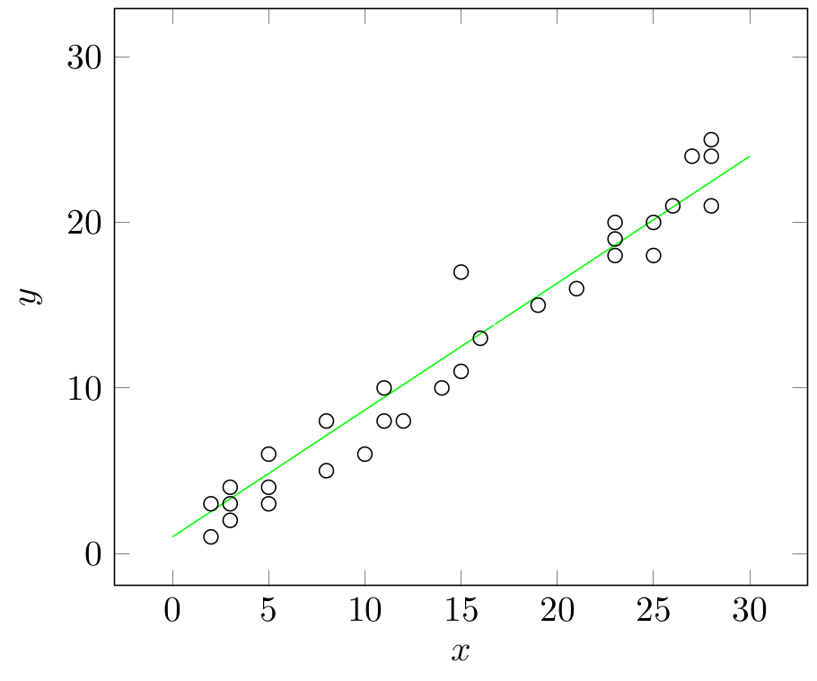
Consider a variable \(y\) which we believe is explained by another variable \(x\) via a linear relationship like:
\[y=\beta_{0}+\beta_{1} x+e\]
in this expression,
\(\beta_0\) stands for the autonomous / unconditional component of \(y\)
\(\beta_{1} x\) stands for the part of \(y\) attributable to \(x\); depending on the sign of \(\beta_{1}\), an increase in \(x\) may induce an increase or a decrease in \(y\)
A case of \(\beta_{1}=0\) corresponds to our unconditional model of mean
Below, the green line is a good candidate to be a Simple Linear regression line:
Notice that we need to estimate two parameters \(\beta_{0}\) and \(\beta_{1}\) this time. The Least squares method is again applicable. Let us go over its steps below:
\[\begin{aligned} & \hat{y}_{i}=\hat{\beta}_{0}+\hat{\beta}_{1} x_{i} \\ & y_{i}=\hat{\beta}_{0}+\hat{\beta}_{1} x_{i}+\hat{e}_{i} \\ & \hat{e}_{i}=y_{i}-\hat{\beta}_{0}-\hat{\beta}_{1} x_{i} \end{aligned}\]
\[\begin{aligned} & S=\sum_{i=1}^{n} \hat{e}_{i}^{2}=\sum_{i=1}^{n}\left(y_{i}-\hat{\beta}_{0}-\hat{\beta}_{1} x_{i}\right)^{2} \\ \end{aligned}\]
\[\begin{aligned} & \min_{\left\{\hat{\beta}_{0}, \hat{\beta}_{1}\right\}} \sum_{i=1}^{n}\left(y_{i}-\hat{\beta}_{0}-\hat{\beta}_{1} x_{i}\right)^{2} \\ \end{aligned}\]
\[\begin{aligned} & \frac{\partial S}{\partial \hat{\beta}_{0}}=\sum_{i=1}^{n} 2\left(y_{i}-\hat{\beta}_{0}-\hat{\beta}_{1} x_{i}\right)(-1)=0 \\ & \frac{\partial S}{\partial \hat{\beta}_{1}}=\sum_{i=1}^{n} 2\left(y_{i}-\hat{\beta}_{0}-\hat{\beta}_{1} x_{i}\right)\left(-x_{i}\right)=0 \\ \end{aligned}\]
\[\begin{aligned} & \sum_{i=1}^{n}\left(y_{i}-\hat{\beta}_{0}-\hat{\beta}_{1} x_{i}\right)=0 \\ & \sum_{i=1}^{n}\left(y_{i}-\hat{\beta}_{0}-\hat{\beta}_{1} x_{i}\right) x_{i}=0 \end{aligned}\]
\[\begin{aligned} & \sum y_{i}-n \hat{\beta}_{0}-\left(\sum x_{i}\right) \hat{\beta}_{1}=0 \\ & \sum x_{i} y_{i}-\left(\sum x_{i}\right) \hat{\beta}_{0}-\left(\sum x_{i}^{2}\right) \hat{\beta}_{1}=0 \\ \end{aligned}\]
\[\begin{aligned} & n \hat{\beta}_{0}+\left(\sum x_{i}\right) \hat{\beta}_{1}=\sum y_{i} \\ & \left(\sum x_{i}\right) \hat{\beta}_{0}+\left(\sum x_{i}^{2}\right) \hat{\beta}_{1}=\sum x_{i} y_{i} \\ \end{aligned}\]
\[\begin{aligned} & \frac{n \sum x_{i}^{2}}{\sum x_{i}} \hat{\beta}_{0}+\left(\sum x_{i}^{2}\right) \hat{\beta}_{1}=\frac{\sum x_{i}^{2} \sum y_{i}}{\sum x_{i}} \\ & \left(\sum x_{i}\right) \hat{\beta}_{0}+\left(\sum x_{i}^{2}\right) \hat{\beta}_{1}=\sum x_{i} y_{i} \\ \end{aligned}\]
\[\begin{aligned} & \left(\frac{n \sum x_{i}^{2}}{\sum x_{i}}-\sum x_{i}\right) \hat{\beta}_{0}=\frac{\sum x_{i}^{2} \sum y_{i}}{\sum x_{i}}-\sum x_{i} y_{i} \\ & \left(\frac{n \sum x_{i}^{2}-\left(\sum x_{i}\right)^{2}}{\sum x_{i}}\right) \hat{\beta}_{0}=\frac{\sum x_{i}^{2} \sum y_{i}-\sum x_{i} \sum x_{i} y_{i}}{\sum x_{i}} \\ \end{aligned}\]
\[\begin{aligned} & \hat{\beta}_{0}=\frac{\sum x_{i}^{2} \sum y_{i}-\sum x_{i} \sum x_{i} y_{i}}{n \sum x_{i}^{2}-\left(\sum x_{i}\right)^{2}} \end{aligned}\]
\[\begin{aligned} & \sum y_{i}-n \hat{\beta}_{0}-\left(\sum x_{i}\right) \hat{\beta}_{1}=0 \\ & n \hat{\beta}_{0}=\sum y_{i}-\left(\sum x_{i}\right) \hat{\beta}_{1}=0 \\ & \hat{\beta}_{0}=\bar{y}-\bar{x} \hat{\beta}_{1} \\ & \hat{\beta}_{0}=\bar{y}-\hat{\beta}_{1} \bar{x} \end{aligned}\]
\[\begin{aligned} & \sum x_{i} y_{i}-\left(\sum x_{i}\right)\left(\bar{y}-\hat{\beta}_{1} \bar{x}\right)-\left(\sum x_{i}^{2}\right) \hat{\beta}_{1}=0 \\ & \sum x_{i} y_{i}-\bar{y} \sum x_{i}-\hat{\beta}_{1} \bar{x} \sum x_{i}-\hat{\beta}_{1} \sum x_{i}^{2}=0 \\ & \frac{\sum x_{i} y_{i}}{n}-\bar{y} \frac{\sum x_{i}}{n}-\hat{\beta}_{1} \bar{x} \frac{\sum x_{i}}{n}-\hat{\beta}_{1} \frac{\sum x_{i}^{2}}{n}=0 \\ & \frac{\sum x_{i} y_{i}}{n}-\bar{x} \bar{y}-\hat{\beta}_{1} \bar{x}^{2}-\hat{\beta}_{1} \frac{\sum x_{i}^{2}}{n}=0 \\ \end{aligned}\]
\[\begin{aligned} \hat{\beta}_{1}=&\frac{\frac{\sum x_{i} y_{i}}{n}-\bar{x} \bar{y}}{\bar{x}^{2}+\frac{\sum x_{i}^{2}}{n}}\\ =&\frac{n \sum x_{i} y_{i}-n^{2} \bar{x} \bar{y}}{n^{2} \bar{x}^{2}+n \sum x_{i}^{2}} \\ \end{aligned}\]
\[\begin{aligned} \hat{\beta}_{1}=&\frac{n \sum x_{i} y_{i}-\sum x_{i} \sum y_{i}}{n \sum x_{i}^{2}+\left(\sum x_{i}\right)^{2}} \end{aligned}\]
Now, reconsider that \(\hat{\beta}_{0}=\bar{y}-\hat{\beta}_{1} \bar{x}\) and that \(\sum x_{i} y_{i}-\hat{\beta}_{0} \sum x_{i}-\hat{\beta}_{1}\sum x_{i}^{2}=0\). Substituting the first one into the second:
\[\begin{aligned} \sum x_{i}y_{i}-\sum x_{i} \bar{y}+\hat{\beta}_{1} \sum x_{i} \bar{x}-\hat{\beta}_{1} \sum x_{i}^{2}=&0\\ \hat{\beta}_{1}\left(\sum x_{i}^{2}-\sum x_{i} \bar{x}\right)=&\sum x_{i}\left(y_{i}-\bar{y}\right) \\ \hat{\beta}_{1}\sum x_{i}\left(x_{i}-\bar{x}\right)=&\sum x_{i}\left(y_{i}-\bar{y}\right)\\ \hat{\beta}_{1}=&\frac{\sum x_{i}\left(y_{i}-\bar{y}\right)}{\sum x_{i}\left(x_{i}-\bar{x}\right)}\\ \end{aligned}\]
Now notice the following:
\[\begin{aligned} \sum\left(x_{i}-\bar{x}\right)\left(y_{i}-\bar{y}\right)=\sum\left(x_{i}-\bar{x}\right)y_{i}=\sum\left(y_{i}-\bar{y}\right) x_{i} \end{aligned}\]
as,
\[\begin{aligned} \sum\left(x_{i}-\bar{x}\right)\left(y_{i}-\bar{y}\right)=\sum\left(x_{i}-\bar{x}\right) y_{i}-\bar{y}\underbrace{\sum\left(x_{i}-\bar{x}\right)}_{0}=\sum\left(y_{i}-\bar{y}\right) x_{i}-\bar{x}\underbrace{\sum\left(y_{i}-\bar{y}\right)}_{0} \end{aligned}\]
and, as the sum of the deviations from the mean is zero, i.e.,
\[\sum\left(x_{i}-\bar{x}\right)=\sum x_{i}-\sum \bar{x}=\sum x_{i}-n \bar{x}=0\]
and
\[\sum\left(y_{i}-\bar{y}\right)=\sum y_{i}-\sum \bar{y}=\sum y_{i}-n \bar{y}=0\]
The same logic applies in:
\[\begin{aligned} \sum\left(x_{i}-\bar{x}\right)^{2}=&\sum\left(x_{i}-\bar{x}\right)\left(x_{i}-\bar{x}\right)\\ =&\sum\left(x_{i}-\bar{x}\right) x_{i}-\bar{x}\underbrace{\sum\left(x_{i}-\bar{x}\right)}_{0} \end{aligned}\]
At the end, the above-driven expression for \(\hat{\beta}_{1}\), i.e.,
\[\begin{aligned} \hat{\beta}_{1}=&\frac{\sum x_{i}\left(y_{i}-\bar{y}\right)}{\sum x_{i}\left(x_{i}-\bar{x}\right)}\\ \end{aligned}\]
can be rewritten as:
\[\begin{aligned} \hat{\beta}_{1}=&\frac{\sum\left(x_{i}-\bar{x}\right)\left(y_{i}-\bar{y}\right)}{\sum\left(x_{i}-\bar{x}\right)^{2}} \end{aligned}\]
so, can be written as:
\[\hat{\beta}_{1}=\frac{\frac{1}{n} \sum\left(x_{i}-\bar{x}\right)\left(y_{i}-\bar{y}\right)}{\frac{1}{n} \sum\left(x_{i}-\bar{x}\right)^{2}}=\frac{Cov(x,y)}{\operatorname{Var}\left(x\right)}\]
To sum up, our Least Squares estimators \(\hat{\beta}_{0}\) and \(\hat{\beta}_{1}\) for the model parameters \(\beta_0\) and \(\beta_1\) are found to be:
\[\begin{aligned} \hat{\beta}_{1}=&\frac{\sum\left(x_{i}-\bar{x}\right)\left(y_{i}-\bar{y}\right)}{\sum\left(x_{i}-\bar{x}\right)^{2}}=\frac{Cov(x,y)}{\operatorname{Var}\left(x\right)} \end{aligned}\]
and
\[\begin{aligned} \hat{\beta}_{0}=\bar{y}-\hat{\beta}_{1} \bar{x} \end{aligned}\]
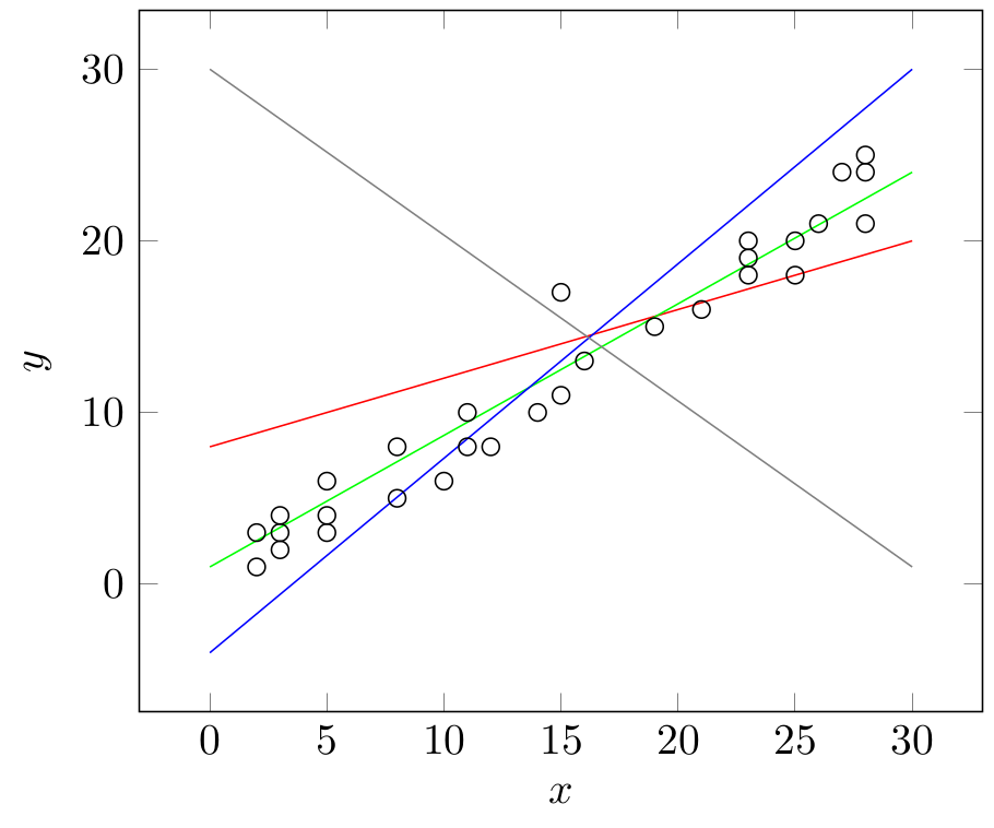
In the graph given below, try to observe why the green line is superior to others in representing our data:
Building and estimating a Multiple Linear Regression model: An increase in dimensionality
Consider \[y=\beta_{0}+\beta_{1} x_{1}+\beta_{2} x_{2}+\cdots+\beta_{k} x_{k}+e\] where
\(\beta_0\) stands for the autonomous/ unconditional component of \(y\)
Each \(\beta_{j} x_{j}\) stands for the part of \(y\) attributable to \(x_{j}\), sign of \(\beta_{j}\) determining the impact of \(x_{j}\) on \(y\). \((j=1,2, \ldots, K)\)
Note again, a case of \(\beta_{1}=\beta_{2}=\ldots=\beta_{K}=0\) corresponds to our unconditional model of mean
\[\begin{aligned} & \hat{y}_{i}=\hat{\beta}_{0}+\hat{\beta}_{1} x_{i 1}+\hat{\beta}_{2} x_{i 2}+\cdots+\hat{\beta}_{K} x_{i K} \\ & y_{i}=\hat{\beta}_{0}+\hat{\beta}_{1} x_{i 1}+\hat{\beta}_{2} x_{i 2}+\cdots+\hat{\beta}_{K} x_{i K}+\hat{e}_{i} \\ & \hat{e}_{i}=y_{i}-\hat{\beta}_{0}-\hat{\beta}_{1} x_{i 1} \cdots+-\hat{\beta}_{K} x_{i K} \end{aligned}\]
\[\begin{aligned} & S=\sum_{i=1}^{n} \hat{e}_{i}^{2}=\sum_{i=1}^{n}\left(y_{i}-\hat{\beta}_{0}-\hat{\beta}_{1} x_{i 1}-\cdots-\hat{\beta}_{K} x_{i K}\right)^{2} \\ & \left\{\hat{\beta}_{0}, \hat{\beta}_{1}, \cdots, \hat{\beta}_{K}\right\} \end{aligned}\]
As before, this minimization problem will give us \(\hat{\beta}_{0}, \hat{\beta}_{1}, \ldots, \hat{\beta}_{K}\), ie., the estimators of \(\beta_0\), \(\beta_1, \ldots, \beta_K\).
For future ease, let us restate our Multiple Linear model using matrix notation. To do this, let us first write our model equation for every single observation (for each \(i=1,2, \ldots, n\)): \[\begin{aligned} & y_{1}=\beta_{0}+\beta_{1} x_{11}+\beta_{2} x_{12}+\cdots+\beta_{K} x_{1 K}+e_{1} \\ & y_{2}=\beta_{0}+\beta_{1} x_{21}+\beta_{2} x_{22}+\cdots+\beta_{K} x_{2 K}+e_{2} \\ & \quad \quad \quad \cdots \quad \quad \quad \cdots \quad \quad \quad \cdots \\ & y_{n}=\beta_{0}+\beta_{1} x_{n 1}+\beta_{2} x_{n 2}+\cdots+\beta_{K} x_{n K}+e_{n} \end{aligned}\]
In matrix notation: \[\underbrace{\left[\begin{array}{c} y_{1} \\ y_{2} \\ \vdots \\ \vdots \\ y_{n} \end{array}\right]}_{y_{(n\times1)}}= \underbrace{\left[\begin{array}{ccccc} 1 & x_{11} & x_{12} & \cdots & x_{1K} \\ 1 & x_{21} & x_{22} & & x_{2K} \\ \vdots & & & & \\ 1 & x_{n1} & x_{n2} & \cdots & x_{nK} \end{array}\right]}_{X_{(n\times(K+1))}} \underbrace{\left[\begin{array}{c} \beta_{0} \\ \beta_{1} \\ \vdots \\ \beta_{K} \end{array}\right]}_{\beta_{((K+1)\times 1)}}+ \underbrace{\left[\begin{array}{c} e_{1} \\ e_{2} \\ \vdots \\ \vdots \\ e_{n} \end{array}\right]}_{e_{(n\times1)}}\] can be written. Then, \[y=X \beta+e\]
It is also possible to write each explanatory variable as a separate vector like: \[x_{0}=\left[\begin{array}{l} 1 \\ 1 \\ 1 \\ \vdots \\ 1 \end{array}\right], x_{1}=\left[\begin{array}{c} x_{11} \\ x_{21} \\ \vdots \\ \vdots \\ x_{n 1} \end{array}\right], \ldots, x_{K}=\left[\begin{array}{c} x_{1 K} \\ x_{2 K} \\ \vdots \\ \vdots \\ x_{n K} \end{array}\right]\] so the model looks like: \[y=x_{0} \beta_{0}+x_{1} \beta_{1}+\cdots+x_{K} \beta_{K}+e\]
When the matrix expression \(y=X \beta+e\) is maintained, the function \(S\) becomes \[S=e^{\prime} e\] where \(e^{\prime}\) is the transpose of \(e\).
Returning to our minimization problem written in classical notation, the following first order conditions are written: \[\begin{aligned} & \frac{\partial S}{\partial \hat{\beta}_{0}}=\sum_{i=1}^{n}-2\left(y_{i}-\hat{\beta}_{0}-\hat{\beta}_{1} x_{i 1} \cdots-\hat{\beta}_{K} x_{i K}\right)=0 \\ & \frac{\partial S}{\partial \hat{\beta}_{1}}=\sum_{i=1}^{n}-2\left(y_{i}-\hat{\beta}_{0}-\hat{\beta}_{1} x_{i 1}-\cdots-\hat{\beta}_{K} x_{i K}\right) x_{i 1}=0 \\ & \quad \quad \quad \cdots \quad \quad \quad \cdots \quad \quad \quad \cdots \\& \frac{\partial S}{\partial \hat{\beta}_{K}}=\sum_{i=1}^{n}-2\left(y_{i}-\hat{\beta}_{0}-\hat{\beta}_{1} x_{i 1}-\cdots-\hat{\beta}_{K} x_{i K}\right) x_{i K}=0 \end{aligned}\]
Simplifying a little: \[\begin{aligned} & \sum\left(y_{i}-\hat{\beta}_{0}-\hat{\beta}_{1} x_{i 1}-\cdots-\hat{\beta}_{K} x_{i K}\right)=0 \\ & \sum\left(y_{i}-\hat{\beta}_{0}-\hat{\beta}_{1} x_{i 1}-\cdots-\hat{\beta}_{K} x_{i K}\right) x_{i 1}=0 \\ & \quad \quad \quad \cdots \quad \quad \quad \cdots \quad \quad \quad \cdots \\ & \sum\left(y_{i}-\hat{\beta}_{0}-\hat{\beta}_{1} x_{i 1}-\cdots-\hat{\beta}_{K} x_{i K}\right) x_{i K}=0 \end{aligned}\]
Reorganizing the terms: \[\begin{gathered} n \hat{\beta}_{0}+\sum x_{i 1} \hat{\beta}_{1}+\cdots+\sum x_{i K} \hat{\beta}_{K}=\sum y_{i} \\ \sum x_{i 1} \hat{\beta}_{0}+\sum x_{i 1}^{2} \hat{\beta}_{1}+\cdots+\sum x_{i 1} x_{i K} \hat{\beta}_{K}=\sum x_{i 1} y_{i} \\ \quad \quad \quad \cdots \quad \quad \quad \cdots \quad \quad \quad \cdots \\ \sum x_{i K} \hat{\beta}_{0}+\sum x_{i 1} x_{i K} \hat{\beta}_{1}+\cdots+\sum x_{i K}^{2} \hat{\beta}_{k}=\sum x_{i K} y_{i} \end{gathered}\]
Notice that this last set of equations can be written as: \[\left[\begin{array}{cccc} n & \sum x_{i 1} & \cdots & \sum x_{i K} \\ \sum x_{i 1} & \sum x_{i 1}^{2} & & \sum x_{i 1} x_{i K} \\ \vdots & & & \\ \Sigma x_{i K} & \sum x_{i 1} x_{i K} & \cdots & \sum x_{i K}^{2} \end{array}\right]\left[\begin{array}{c} \hat{\beta}_{0} \\ \hat{\beta}_{1} \\ \vdots \\ \vdots \\ \hat{\beta}_{K} \end{array}\right]=\left[\begin{array}{c} \Sigma y_{i} \\ \Sigma x_{i 1} y_{i} \\ \\ \\ x_{i K} y_{i} \end{array}\right]\]
In terms of our earlier definitions of \(x\) and \(y\) as well as \(\beta\); what we have obtained is \[X^{\prime} X \hat{\beta}=X^{\prime} y\]
So, \[\hat{\beta}=\left(X^{\prime} X\right)^{-1} X^{\prime} y\]
Solves our minimization problem and \(\hat{\beta}=\left[\hat{\beta}_{0}, \hat{\beta}_{1}, \hat{\beta}_{2}, \cdots ,\hat{\beta}_{K}\right]^{\prime}\) contains our parameter estimates.
Exercise. Reconsider the Simple Linear model \(y=\beta_{0}+\beta_{1} x+e\) and show that the \(\hat{\beta}=\left(X^{\prime} X\right)^{-1} X^{\prime} y\) works in estimating \(\beta_{0}\) and \(\beta_{1}\) (ie., while finding \(\hat{\beta}_{0}\) and \(\hat{\beta}_{1}\) ).
Solution. \[\begin{aligned} & X^{\prime} X=\left[\begin{array}{cc} n & \Sigma x_{i} \\ \Sigma x_{i} & \Sigma x_{i}^{2} \end{array}\right] \\ & X^{\prime} y=\left[\begin{array}{l} \sum y_{i} \\ \sum x_{i} y_{i} \end{array}\right] \\ & \left(X^{\prime} X\right)^{-1}=\frac{1}{n \sum x_{i}^{2}-\left(\sum x_{i}\right)^{2}} \left[\begin{array}{cc} \sum x_{i}^{2} & -\Sigma x_{i} \\ -\Sigma x_{i} & n \end{array}\right] \end{aligned}\]
So, \[\hat{\beta}=\frac{1}{n \sum x_{i}^{2}-\left(\Sigma x_{i}\right)^{2}}\left[\begin{array}{cc} \Sigma x_{i}^{2} & -\Sigma x_{i} \\ -\Sigma x_{i} & n \end{array}\right]\left[\begin{array}{c} \Sigma y_{i} \\ \Sigma x_{i} y_{i} \end{array}\right]\]
So, \[\begin{aligned} & \hat{\beta}_{0}=\frac{\sum x_{i}^{2} \sum y_{i}-\sum x_{i} \sum x_{i} y_{i}}{n \sum x_{i}^{2}-\left(\sum x_{i}\right)^{2}} \\ & \hat{\beta}_{1}=\frac{-\sum x_{i} \sum y_{i}+n \sum x_{i} y_{i}}{n \sum x_{i}^{2}-\left(\sum x_{i}\right)^{2}}=\frac{n \sum x_{i} y_{i}-\sum x_{i} \sum y_{i}}{n \sum x_{i}^{2}-\left(\sum x_{i}\right)^{2}} \end{aligned}\]
Checking back our earlier solution, we verify that \(\hat{\beta}=\left(X^{\prime} X\right)^{-1} X^{\prime} y\) works well.
Question: Write and solve the Least squares estimation problem for \[y_{i}=\beta_{0}+\beta_{1} x_{i 1}+\beta_{2} x_{i 2}+e_{i}\] that is, a model with a constant term \(\left(\beta_{0}\right)\) and two explanatory variables.
Solution. Solution: Left as self-study.
Goodness of fit
Suppose we have the following model:
\[\begin{aligned} & y_{i}=\overbrace{\hat{\beta}_{0}+\hat{\beta}_{1} x_{i}}^{\hat{y}_{i}}+e_{i}=\hat{y}_{i}+e_{i} \\ \end{aligned}\]
Observe that \[\begin{aligned} & y_{i}-\bar{y}=\hat{y}_{i}-\bar{y}+e_{i} \\ \end{aligned}\]
and consider the quantity \(\sum\left(y_{i}-\bar{y}\right)^{2}\): This quantity is called ’Total Sum of Squares’. In what follows, we decompose it into other useful quantities:
\[\begin{aligned} \sum\left(y_{i}-\bar{y}\right)^{2}=&\sum\left(\hat{y}_{i}-\bar{y}\right)^{2}+2\sum\left(\hat{y}_{i}-\bar{y}\right)e_{i}+\sum e_{i}^{2}\\ \end{aligned}\]
Reordering the terms in the last expression:
\[\begin{aligned} \sum\left(y_{i}-\bar{y}\right)^{2}=&\sum(\hat{y}_{i}-\bar{y}+e_{i})^2\\ =&\sum\left(\hat{y}_{i}-\bar{y}\right)^{2}+\sum e_{i}^{2}+2\underbrace{\sum\left(\hat{y}_{i}-\bar{y}\right)e_{i}}_{0}\\ \sum\left(y_{i}-\bar{y}\right)^{2}=&\sum\left(\hat{y}_{i}-\bar{y}\right)^{2}+\sum e_{i}^{2}\\ \end{aligned}\]
is obtained. In this expression,
\[\begin{aligned} \underbrace{\sum\left(y_{i}-\bar{y}\right)^{2}}_{TSS}=&\underbrace{\sum\left(\hat{y}_{i}-\bar{y}\right)^{2}}_{ESS}+\underbrace{\sum e_{i}^{2}}_{RSS}\\ \end{aligned}\]
\(TSS\), \(ESS\) and \(RSS\) stand for:
\(TSS\): Total Sum of Squares
\(ESS\): Explained Sum of Squares
\(RSS\): Residual Sum of Squares
Notice that the Total Sum of Squares \(\sum\left(y_{i}-\bar{y}\right)^{2}\) is nothing but the variance of \(y\) multiplied by \(n\) :
\[TSS=\sum\left(y_{i}-\bar{y}\right)^{2}=n\left(\frac{1}{n} \sum\left(y_{i}-\bar{y}\right)^{2}\right)\]
Explained Sum of Squares \(\sum\left(\hat{y}_{i}-\bar{y}\right)^{2}\) measures the sum of squared deviations of our estimated values of \(y\) (namely \(\hat{y}_{i}\) ) from \(\bar{y}\) (namely the unconditional mean of our dependent variable \(y\) ). As \(\hat{y}_{i}\) values are implied by our model’s explanatory variables \(\left(x_{1}, x_{2}, \ldots, x_{K}\right)\), the \(ESS\) measures the portion of \(TSS\) that we explained. Residual Sum of Squares, then, measures the portion of \(TSS\) that could not be explained. The Coefficient of Determination \(R^{2}\) is the fraction of variation in \(y\) explained by our knowledge of \(x\): \[\begin{aligned} R^{2}=\frac{ESS}{TSS}=&\frac{\sum\left(\hat{y}_{i}-\bar{y}\right)^{2}}{\sum\left(y_{i}-\bar{y}\right)^{2}}\\ =&1-\frac{RSS}{TSS} \\ =&1-\frac{\sum \hat{e}_{i}^{2}}{\sum\left(y_{i}-\bar{y}\right)^{2}} \end{aligned}\]
Note that, if the model does not have a constant term (that is \(\beta_{0}\) is omitted), then the measure \(R^{2}\) is not appropriate anymore. When the constant term is omitted, \[\sum\left(y_{i}-\bar{y}\right)^{2} \neq \sum\left(\hat{y}_{i}-\bar{y}\right)^{2}+\sum e_{i}^{2}\]
A bad habit of \(R^{2}\) is that it tends to somehow increase upon the inclusion of additional explanatory variables (in fact, when their t-statistics exceed \(1\) in absolute value: we will see in subsequent sections) in a model. Does this mean we should continue adding more and more explanatory variables to our model ’just to push up \(R^{2}\)’? The answer is quite the opposite: we must see the inclusion of more variables as a cost (after all we want to come up with a parsimonious model). Then, we need to balance the benefits of more explanatory variables (enhanced \(ESS\)) with the cost of including them.
The Adjusted Coefficient of Determination \(\left(\bar{R}^{2}\right)\) serves that purpose: \[\bar{R}^{2}=1-\frac{RSS /(n-K-1)}{TSS/(n-1)}\]
Notice that: \[\bar{R}^{2}=1-\left(1-R^{2}\right)\left(\frac{n-1}{n-K-1}\right)\]
Also keep in mind that neither \(R^{2}\) nor \(\bar{R}^{2}\) has a statistical distribution. So, they are not directly and formally testable. Though, a simple arithmetic reorganization of \(\bar{R}^{2}\) resembles an \(F\) test score (test statistic) as we will consider very soon.
Handling statistical uncertainty: calculation of variances and covariances associated with a Multiple Linear Regression model
As stated before in "Our approach to teaching/learning’, up to here we maintained a naive and mechanical view of the Linear Regression modeling. In that, we deliberately, avoided calculations and discussions of the measures of dispersion or co-dispersion associated with our models. Now, it is the time to turn to reality. After all, \(e_{i}\) sequence has a certain statistical distribution, so does \(y_{i}\). As we will formally study under the heading of ’Ideal econometric conditions: Gauss-Markov assumptions’, the \(e_{i}\) terms have: \[e_{i} \sim \operatorname{Normal}(0, \sigma^{2})\] that is, a Normal (Gaussian) distributton with a mean of zero (\(0\)) and constant (and preferably finite) variance.
As a consequence \(y_i\) values have: \[y_{i} \sim \operatorname{Normal}(\beta_{0}+\beta_{1} x_{1}+\cdots+\beta_{K} x_{K}, \sigma^{2})\]
Intuitively, the mean of \(y_{i}\) depends on (is conditional on) \(x_{1}, x_{2}, \ldots, x_{K}\) (along with their parameters); while variance of \(y\) simply mimics that of \(e\) (by the very construction of our analytical framework).
The key thing to understand now is the variability of our parameter estimates: once they are obtained from a stochastic/ random data set, it is natural/ trivial to expect each of our estimators to have a nonzero variance and each pair of our estimators to have a covariance.
We devote this section to some rigorous treatment of what we call a ’variance-covariance’ matrix.
Let us begin from \(e \sim \operatorname{Normal}(0, \sigma^{2})\). Once we assume the error terms to have a Normal distribution with a mean of zero (\(0\)) and a variance of \(\sigma^{2}\), we may proceed to the following Q&A style mathematical elaboration:
Q: Do we know the value of \(\sigma^{2}\) ?
A: No, it belongs to the population of \(e_i\)’s. But, we only have a sample of \(e_{i}\) ’s, namely \(\hat{e}_{i}\) ’s.
Q: Can we use those \(\hat{e}_{i}\) ’s to estimate \(\sigma^{2}\), that is to obtain \(\hat{\sigma}^{2}\) ?
A: Yes, the formula for \(\hat{\sigma}^{2}\) is: \[\hat{\sigma}^{2}=\frac{\sum \hat{e}_{i}^{2}}{n-(K+1)}\]
Q: can we express \(\hat{\sigma}^{2}\) using matrix notation?
A: Yes, the expression is: \[\hat{\sigma}^{2}=\frac{\hat{e}^{\prime} \hat{e}}{n-(K+1)}=\frac{(y-X \beta)^{\prime}(y-X \beta)}{n-(K+1)}\]
Q: What about the \(Cov\left(\hat{\beta}_{i}, \hat{\beta}_{j}\right)\) values, can we calculate them?
A: Sure, in matrix notation, \[Cov(\hat{\beta})=\operatorname{E}\!\left((\hat{\beta}-\beta)(\hat{\beta}-\beta)^{\prime}\right)=\sigma^{2}\left(X^{\prime} X\right)^{-1}\]
Q: What about the distribution of \(\hat{\beta}\) ?
A: \[\hat{\beta} \sim \operatorname{Normal}(\beta, \sigma^{2}\left(X^{\prime} X)^{-1}\right)\]
Q: What does this mean?
A: First, each parameter estimate is unbiased, \(\operatorname{E}\!\left(\hat{\beta}\right)=\beta\). Second, the variances are ruled by \(\sigma^{2}\left(X^{\prime}X\right)^{-1}\).
Q: How is the structure of the variance-covariance matrix?
A: \[\begin{aligned} \operatorname{Cov}(\hat{\beta}) &= \operatorname{E}\!\left((\hat{\beta}-\beta)\left(\hat{\beta}-\beta\right)^{\prime}\right) \\ &=\left[\begin{array}{ccc} \operatorname{Var}\left(\hat{\beta}_{0}\right) Cov\left(\hat{\beta}_{0}, \hat{\beta}_{1}\right) & \cdots & Cov\left(\hat{\beta}_{0}, \hat{\beta}_{K}\right) \\ Cov\left(\hat{\beta}_{0}, \hat{\beta}_{1}\right) \operatorname{Var}\left(\hat{\beta}_{1}\right) & \cdots & Cov\left(\hat{\beta}_{1}, \hat{\beta}_{K}\right) \\ \quad \cdots \quad & \quad \cdots \quad & \quad \cdots \quad \\ Cov\left(\hat{\beta}_{0}, \hat{\beta}_{K}\right) Cov\left(\hat{\beta}_{1}, \hat{\beta}_{K}\right) & \cdots & \operatorname{Var}\left(\hat{\beta}_{K}\right) \end{array}\right] \end{aligned}\]
\[\begin{aligned} & =\left[\begin{array}{cccc} E\left(\hat{\beta}_{0}-\beta_{0}\right)^{2} & E\left(\hat{\beta}_{0}-\beta_{0}\right)\left(\hat{\beta}_{1}-\beta_{1}\right) & \cdots & E\left(\hat{\beta}_{0}-\beta_{0}\right)\left(\hat{\beta}_{K}-\beta_{K}\right) \\ E\left(\hat{\beta}_{0}-\beta_{0}\right)\left(\hat{\beta}_{1}-\beta_{1}\right) & E\left(\hat{\beta}_{1}-\beta_{1}\right)^{2} & \cdots & E\left(\hat{\beta}_{1}-\beta_{1}\right)\left(\hat{\beta}_{K}-\beta_{K}\right) \\ & & & \\ E\left(\hat{\beta}_{0}-\beta_{0}\right)\left(\hat{\beta}_{K}-\beta_{K}\right) & E\left(\hat{\beta}_{1}-\beta_{1}\right)\left(\hat{\beta}_{K}-\beta_{K}\right) & \cdots & E\left(\hat{\beta}_{K}-\beta_{K}\right)^{2} \end{array}\right] \\ & =\sigma^{2}\left(X^{\prime} X\right)^{-1}=\sigma^{2}\left[\begin{array}{cccc} n & \sum x_{i 1} & \cdots & \Sigma_{x_{i K}} \\ \Sigma x_{i 1} & \Sigma x_{i 1}^{2} & \cdots & \Sigma_{x_{i 1} x_{i K}} \\ \vdots & & & \\ \Sigma x_{i K} & \Sigma x_{i 1} x_{i K} & \cdots & \Sigma x_{i K}^{2} \end{array}\right]^{-1} \end{aligned}\]
Q: But, we do not know the value of \(\sigma^{2}\)?
A: Then, substitute \(\hat{\sigma}^{2}\) for it: \[\hat{\operatorname{Cov}}(\beta)=\hat{\sigma}^{2}\left(X^{\prime} X\right)^{-1}\]
Q: Does that mean we will be using the estimated values of variances and covariances?
A: Sure. This is what we have been doing since the beginning of our ECON 222 journey.
Q: Are we now ready to dive into the fascinating world of statistical inference over our estimated models?
A: Very much, indeed.
Q: Are you an AI?
A: No. Are you?
Statistical inference
We have studied/learned up to this point:
Probability basics and a rich-enough collection of well-known statistical distributions in ECON 221 (Chapter 1, Chapter 2, Chapter 3, chapter 4)
Point estimators of distributional parameters, and the fundamentals of statistical inference (confidence intervals and hypothesis testing) in ECON 222 (Chapter 5, Chapter 6, Chapter 7)
Structure, formation and estimation of Simple Linear Regression and Multiple Linear Regression models in ECON 222 (earlier sections of Chapter 8)
Now, we are ready to place our estimated models under some serious scrutiny. Using the inferential tools that we learned, we will evaluate, test and scientifically question our regression models.
In a bold fashion, we can say that what we did up to here (i.e., estimating regression models) is no more than the half of the job. To have the job actually done, we need to delve into the following tasks:
Estimating confidence intervals for individual model parameters \(\beta_{i}\)
Estimating confidence intervals for linear combinations of (more than one) model parameters
Conducting hypothesis tests for individual model parameters \(\beta_{i}\)
Conducting hypothesis tests for linear combinations of (more than one) model parameters
Conducting hypothesis tests for all of our model parameters at once
Conducting hypothesis tests for specific subsets of our model parameters at once
Now, let us give examples to each category of tasks listed above. To do this, suppose we have the following economic model: \[y_{i}=\beta_{0}+\beta_{1} x_{i 1}+\beta_{2} x_{i 2}+\beta_{3} x_{i 3}+\beta_{4} x_{i 4}\]
Recall that, this is our model written for the population and we turn it into a statistical model (written again for the population) by introducing the statistical error (disturbance, sometimes ’shock’) terms: \[y_{i}=\beta_{0}+\beta_{1} x_{i 1}+\beta_{2} x_{i 2}+\beta_{3} x_{i 3}+\beta_{4} x_{i 4}+e_{i}\] where \(e_i \sim \operatorname{Normal}(0, \sigma^{2})\). As you know well now, we do not know the true values (population values of \(\beta_j\) ’s). So, we will estimate the model using a sample of \(n\) observations and the Least Squares technique.
\[\begin{aligned} & y_{i}=\beta_{0}+\beta_{1} x_{i 1}+\beta_{2} x_{i 2}+\beta_{3} x_{i 3}+\beta_{4} x_{i 4}+e_{i}, \\ & \qquad i=1,2, \ldots, n, e_{i} \sim \operatorname{Normal}\left(0, \sigma^{2}\right) \end{aligned}\]
Provided that everything goes well on the paper and in the computer, we will end up with a rich set of estimates:
Estimates of model parameters: \(\hat{\beta}_{0}\), \(\hat{\beta}_{1}\), \(\hat{\beta}_{2}\), \(\hat{\beta}_{3}\), \(\hat{\beta}_{4}\)
Estimated sequence of the dependent variable: \(\hat{y}_{i}\)
Estimated sequence of error terms: \(\hat{e}_{i}\)
Estimated model variance: \[\hat{\sigma}^{2}=\frac{\hat{e}^{\prime} \hat{e}}{n-(K+1)} \quad \left(\text{here, }\frac{\hat{e}^{\prime} \hat{e}}{n-5}\right)\]
Estimated "variance-covariance matrix: \[\hat{Cov}(\beta)=\hat{\sigma}^{2}\left(X^{\prime} X\right)^{-1}\]
Now, suppose the following claims and/or questions come from an academic/ technical colleague. (Needless to say, even when there is no criticizing colleague around, we need to put these claims on our own and heavily test our models):
Is \(0.4\) a viable value for \(\beta_{1}\), with respect to a \(95 \%\) confidence interval of \(\beta_{1}\) ?
Is \(0.7\) a viable value for \(\beta_{1}+\beta_{2}\), with respect to a \(95 \%\) confidence interval of \(\beta_{1}+\beta_{2}\) ?
Is \(\beta_{3}\) equal zero or not; how do we know \(x_{3}\) is an important/significant explanatory variable?
Is \(\beta_{3}+\beta_{4}\) equal one or not?
Is \(\beta_{1}=\beta_{2}=\beta_{3}=\beta_{4}=0\); how do we know our explanatory variables \(x_{1}, x_{2}, x_{3}\) and \(x_{4}\) matter as a whole?
Is \(\beta_{1}=\beta_{2}=0\); how do we know the explanatory variables \(x_{1}\) and \(x_{2}\) matter together?
Our road map to assess these questions begins with formulating these questions/claims in some formal notation:
Following the same order as above:
We will calculate a \(95 \%\) C.I. for \(\beta_{1}\) and will check if \(0.4\) belongs to the calculated interval. This is simply done as: \[\operatorname{P}\!\left(\hat{\beta}_{1}-t_{c} \operatorname{se}\left(\hat{\beta}_{1}\right) \leq \beta_{1} \leq \hat{\beta}_{1}+t_{c} \operatorname{se}\left(\hat{\beta}_{1}\right)\right)=1-\alpha\]
We will calculate a \(95 \%\) C.1. for \(\beta_{1}+\beta_{2}\) and will check if \(0.7\) belongs to the calculated interval. \[\operatorname{P}\!\left(\hat{\beta}_{1}+\hat{\beta}_{2}-t_{c} \operatorname{se}\left(\hat{\beta}_{1}+\hat{\beta}_{2}\right) \leq \beta_{1}+\beta_{2} \leq \hat{\beta}_{1}+\hat{\beta}_{2}+t_{c} \operatorname{se}\left(\hat{\beta}_{1}+\hat{\beta}_{2}\right)\right)=1-\alpha\] Here, we apparently need to calculate \(\operatorname{Var}\left(\hat{\beta}_{1}+\hat{\beta}_{2}\right)\). Using our knowledge from ECON 221: \[\operatorname{Var}\left(\hat{\beta}_{1}+\hat{\beta}_{2}\right)=\operatorname{Var}\left(\hat{\beta}_{1}\right)+2Cov(\hat{\beta}_{1},\hat{\beta}_{2})+\operatorname{Var}\left(\hat{\beta}_{2}\right)\] where \(\operatorname{Var}\left(\hat{\beta}_{1}\right)\), \(Cov(\hat{\beta}_{1},\hat{\beta}_{2})\) and \(\operatorname{Var}\left(\hat{\beta}_{2}\right)\) are straightforwardly obtained during the estimation of the model. Once \(\operatorname{Var}\left(\hat{\beta}_{1}+\hat{\beta}_{2}\right)\) is at hand, \(se(\hat{\beta}_{1}+\hat{\beta}_{2})=\sqrt{\operatorname{Var}\left(\hat{\beta}_{1}+\hat{\beta}_{2}\right)}\) yields the required standard error.
We will conduct the test \[\begin{aligned} & H_{0}: \beta_{3}=0 \\ & H_{1}: \beta_{3} \neq 0 \end{aligned}\] Distribution of the test statistic: \[\begin{aligned} & \frac{\hat{\beta}_{3}-\beta_{3}}{\sqrt{\operatorname{Var}\left(\hat{\beta}_{3}\right)}} \sim t_{(n-K-1)} \end{aligned}\] Calculation of the test statistic: \[\begin{aligned} & \frac{\hat{\beta}_{3}-\beta_{3}^{0}}{\operatorname{se}\left(\hat{\beta}_{3}\right)} \sim t_{(n-K-1)} \\ \end{aligned}\] \[\begin{aligned} & \frac{\hat{\beta}_{3}-0}{\operatorname{se}\left(\hat{\beta}_{3}\right)} \sim t_{(n-K-1)} \\ \end{aligned}\]
We will conduct the test \[\begin{aligned} & H_{0}: \beta_{3}+\beta_{4}=1 \\ & H_{1}: \beta_{3}+\beta_{4} \neq 1 \end{aligned}\] \[\begin{aligned} & \frac{\hat{\beta}_{3}+\hat{\beta}_{4}-(\beta_{3}+\beta_{4})}{\sqrt{\operatorname{Var}\left(\hat{\beta}_{3}+\hat{\beta}_{4}\right)}} \sim t_{(n-K-1)} \end{aligned}\] \[\begin{aligned} & \frac{\hat{\beta}_{3}+\hat{\beta}_{4}-(\beta_{3}+\beta_{4})^{0}}{\operatorname{se}\left(\hat{\beta}_{3}+\hat{\beta}_{4}\right)} \sim t_{(n-K-1)} \\ \end{aligned}\] \[\begin{aligned} & \frac{\hat{\beta}_{3}+\hat{\beta}_{4}-1}{\operatorname{se}\left(\hat{\beta}_{3}+\hat{\beta}_{4}\right)} \sim t_{(n-K-1)} \\ \end{aligned}\] \(\operatorname{Var}\left(\hat{\beta}_{3}+\hat{\beta}_{4}\right)\) will be treated as outlined above for the case of \(\operatorname{Var}\left(\hat{\beta}_{1}+\hat{\beta}_{2}\right)\). Note that this test can also be conducted as an \(F\) test, as we will cover in our class discussions.
We will conduct the test \[\begin{array}{ll} H_{0}: & \beta_{1}=\beta_{2}=\beta_{3}=\beta_{4}=0 \\ H_{1}: & \exists \beta_{i} \neq 0 \end{array}\] Total sum of squares \(TSS\) being \(\sum\left(y_{i}-\bar{y}\right)^{2}\), explained sum of squares \(ESS\) being \(\sum\left(\hat{y}_{i}-\bar{y}\right)^{2}\) and residual sum of squares \(RSS\) being \(\sum\hat{e}_{i}^{2}\): \[\frac{(TSS-RSS)/K}{RSS/(n-K-1)} \sim F_{(K, n-K-1)}\]
We will conduct the test \[\begin{aligned} H_{0}:& \beta_{1}=\beta_{2}=0 \\ H_{1}:& \beta_{1} \neq 0 \text{ or } \beta_{2} \neq 0 \end{aligned}\] \(J\) being the number of joint hypotheses, \(RSS_R\) being the \(RSS\) for the restricted model and \(RSS_U\) being the \(RSS\) for the unrestricted model: \[\frac{\left(RSS_{R}-RSS_{U}\right)/J}{RSS_{U}/(n-K-1)} \sim F_{(J,n-K-1)}\] Note / clarify again that \(RSS_{U}\) is the \(RSS\) value of the unrestricted, i.e., full model, which is: \[y_{i}=\beta_{0}+\beta_{1} x_{i 1}+\beta_{2} x_{i 2}+\beta_{3} x_{i 3}+\beta_{4} x_{i 4}+e_{i}\] where, \(RSS_{R}\) is the \(RSS\) value of the restricted model, which is: \[y_{i}=\beta_{0}+\beta_{3} x_{i 3}+\beta_{4} x_{i 4}+e_{i}\] equivalently of: \[y_{i}=\beta_{0}+0\cdot x_{i 1}+0\cdot x_{i 2}+\beta_{3} x_{i 3}+\beta_{4} x_{i 4}+e_{i}\]
Returning to our previous hypothesis test: \[\begin{array}{ll} H_{0}: & \beta_{1}=\beta_{2}=\beta_{3}=\beta_{4}=0 \\ H_{1}: & \exists \beta_{i} \neq 0 \end{array}\] you will notice that the restricted model is: \[y_{i}=\beta_{0}+e_{i}\] or \[y_{i}=\beta_{0}+0\cdot x_{i 1}+0\cdot x_{i 2}+0\cdot x_{i 3}+0\cdot x_{i 4}+e_{i}\] against the unrestricted (full) model of: \[y_{i}=\beta_{0}+\beta_{1} x_{i 1}+\beta_{2} x_{i 2}+\beta_{3} x_{i 3}+\beta_{4} x_{i 4}+e_{i}\] Herein, \(RSS_{R}\) becomes the \(TSS\) of the full model (verify yourself), \(RSS_{U}\) becomes the \(RSS\) of the full model (should be trivial) and \(J\) becomes \(K\). Then, the equivalence between \[\frac{\left(RSS_{R}-RSS_{U}\right)/J}{RSS_{U}/(n-K-1)}\sim F_{(J,n-K-1)}\] and \[\frac{(TSS-RSS)/K}{RSS/(n-K-1)}\sim F_{(K,n-K-1)}\] becomes apparent.
We will now use a model estimated on a computer to exemplify each of the cases above:
[To be distributed as a handout]
Essence of the Gauss-Markov assumptions
Having studied the mechanical aspects of Linear Regression models, now it is the time to establish the conditions under which a linear regression model is viable with workable results. As we often call it ’ideal econometric conditions’, the Gauss-Markov assumptions level the field for us. If a model abides by these assumptions, i.e., if a model has been formed so as to hold the Gauss-Markov assumptions, then it is a good econometric model.
Now we can review how good is our LS estimator under these conditions. Consider the Simple Linear regression model \(y_{i}=\beta_{0}+\beta_{1} x_{i}+e_{i}\) and consider the Gauss-Markov assumptions. Let us now try to see how good is our LS estimator under these assumptions. Recall that \(\hat{\beta}_{1}\) is:
\[\hat{\beta}_{1}=\frac{\sum\left(x_{i}-\bar{x}\right)\left(y_{i}-\bar{y}\right)}{\sum\left(x_{i}-\bar{x}\right)^{2}}\]
which can also be written as:
\[\begin{aligned} \hat{\beta}_{1} & =\frac{\sum\left(x_{i}-\bar{x}\right) y_{i}}{\sum\left(x_{i}-\bar{x}\right) x_{i}} \\ & =\frac{\sum\left(x_{i}-\bar{x}\right)\left(\beta_{0}+\beta_{1} x_{i}+e_{i}\right)}{\sum\left(x_{i}-\bar{x}\right) x_{i}} \\ & =\frac{\beta_{0} \sum\left(x_{i}-\bar{x}\right)+\beta_{1} \sum\left(x_{i}-\bar{x}\right) x_{i}+\sum\left(x_{i}-\bar{x}\right) e_{i}}{\sum\left(x_{i}-\bar{x}\right) x_{i}} \end{aligned}\]
As \(\sum\left(x_{i}-\bar{x}\right)=0\) (shown before), the expression becomes:
\[\begin{aligned} \hat{\beta}_{1} & =\beta_{1}+\frac{\sum\left(x_{i}-\bar{x}\right) e_{i}}{\sum\left(x_{i}-\bar{x}\right) x_{i}} \\ & =\beta_{1}+\frac{\sum\left(x_{i}-\bar{x}\right) e_{i}}{\sum\left(x_{i}-\bar{x}\right)^{2}} \end{aligned}\]
Then,
\[\begin{aligned} E\left(\hat{\beta}_{1} \mid x\right) & =E\left(\left.\beta_{1}+\frac{\sum\left(x_{i}-\bar{x}\right) e_{i}}{\sum\left(x_{i}-\bar{x}\right)^{2}} \right\rvert\, x\right) \\ & =\beta_{1}+E\left(\left.\frac{\sum\left(x_{i}-\bar{x}\right) e_{i}}{\sum\left(x_{i}-\bar{x}\right)^{2}} \right\rvert\, x\right) \\ & =\beta_{1}+\frac{\sum\left(x_{i}-\bar{x}\right) E\left(e_{i} \mid x\right)}{\sum\left(x_{i}-\bar{x}\right)^{2}} \end{aligned}\]
can be written since our \(x\) (independent variable, explanatory variable) is non-stochastic.
We also know by the Gauss-Markov assumptions that \(E\left(e_{i} \mid x\right)=0\), i.e., our knowledge of \(x\) does not improve expectation of \(e\). So,
\[E\left(\hat{\beta}_{1} \mid x\right)=\beta_{1}\]
equivalently saying \(\hat{\beta}_{1}\) is an unbiased estimator of \(\beta_{1}\).
What about \(E\left(\hat{\beta}_{0} \mid x\right)\) ?
\[\begin{aligned} y_{i} & =\beta_{0}+\beta_{1} x_{i}+e_{i} \rightarrow \bar{y}=\beta_{0}+\beta_{1} \bar{x}+\bar{e} \\ \hat{\beta}_{0} & =\bar{y}-\hat{\beta}_{1} \bar{x} \\ & =\beta_{0}+\beta_{1} \bar{x}+\bar{e}-\hat{\beta}_{1} \bar{x} \\ & =\beta_{0}-\left(\hat{\beta}_{1}-\beta_{1}\right) \bar{x}+\bar{e} \end{aligned}\]
Then,
\[\begin{aligned} E\left(\hat{\beta}_{0} \mid x\right) & =E\left(\beta_{0}-\left(\hat{\beta}_{1}-\beta_{1}\right) \bar{x}+\bar{e} \mid x\right) \\ & =\beta_{0}-\bar{x} \underbrace{E\left(\left(\hat{\beta}_{1}-\beta_{1}\right) \mid x\right)}_{0}+\underbrace{E\left(\left.\frac{\sum e_{i}}{n} \right\rvert\, x\right)}_{0} \end{aligned}\]
So,
\[E\left(\hat{\beta}_{0} \mid x\right)=\beta_{0}\]
equivalently saying \(\hat{\beta}_{0}\) is an unbiased estimator of \(\beta_{0}\).
\[\begin{aligned} \operatorname{Var}\left(\hat{\beta}_{1}\right) & =\operatorname{E}\!\left((\hat{\beta}_{1}-\underbrace{E\left(\hat{\beta}_{1}\right.}_{\beta_{1}}))^{2}\right) \\ & =E\left(\left(\frac{\sum\left(x_{i}-\bar{x}\right) e_{i}}{\sum\left(x_{i}-\bar{x}\right)^{2}}\right)^{2}\right) \end{aligned}\]
Expanding the expression and rearranging its terms:
\[\begin{aligned} & \operatorname{Var}\left(\hat{\beta}_{1}\right)=E\left(\left.\frac{\sum\left(x_{i}-\bar{x}\right)^{2} e_{i}^{2}+\sum\sum\left(x_{i}-\bar{x}\right)\left(x_{j}-\bar{x}\right) e_{i} e_{j}}{\left(\sum\left(x_{i}-\bar{x}\right)^{2}\right)^{2}} \right\rvert\, x\right) \\ & =\frac{\sum\left(x_{i}-\bar{x}\right)^{2} E\left(e_{i}^{2} \mid x\right)+\sum \sum\left(x_{i}-\bar{x}\right)\left(x_{j}-\bar{x}\right) E\left(e_{i} e_{j} \mid x\right)}{\left(\sum\left(x_{i}-\bar{x}\right)^{2}\right)^{2}} \end{aligned}\]
As \(E\left(e_{i}^{2} \mid x\right)=\sigma^{2}\) and \(E\left(e_{i} e_{j} \mid x\right)=0\),
\[\operatorname{Var}\left(\hat{\beta}_{1}\right)=\frac{\sigma^{2} \sum\left(x_{i}-\bar{x}\right)^{2}}{\left(\sum\left(x_{i}-\bar{x}\right)^{2}\right)^{2}}=\frac{\sigma^{2}}{\sum\left(x_{i}-\bar{x}\right)^{2}}=\frac{\sigma^{2}}{n \operatorname{Var}\left(x\right)}\]
This expression is a Noise/Signal (i.e., a noise-to-signal) ratio expression.
Examining
\[\operatorname{Var}\left(\hat{\beta}_{1}\right)=\frac{\sigma^{2}}{n \operatorname{Var}\left(x\right)}\]
We see that, to decrease \(\operatorname{Var}\left(\hat{\beta}_{1}\right)\), a larger sample size \(n\), a larger \(\operatorname{Var}\left(x\right)\) and a smaller \(\sigma^{2}\) would help. Among these, the researcher’s choice of the sample data affects \(n\) and \(\operatorname{Var}\left(x\right)\). \(\sigma^{2}\), on the other hand, is out of the researcher’s reach.
\[\begin{aligned} & \operatorname{Var}\left(\hat{\beta}_{0}\right)=E\left(\left(\hat{\beta}_{0}-E\left(\hat{\beta}_{0}\right)^{2}\right)\right. \\ As \hat{\beta}_{0} & =\beta_{0}-\left(\hat{\beta}_{1}-\beta_{1}\right) \bar{x}+\bar{e}: \\ \operatorname{Var}\left(\hat{\beta}_{0}\right) & =E\left(\left(\beta_{0}-\left(\hat{\beta}_{1}-\beta_{1}\right) \bar{x}+\bar{e}-E\left(\hat{\beta}_{0}\right)^{2}\right)\right. \\ & =E\left(\left(\beta_{0}-\left(\hat{\beta}_{1}-\beta_{1}\right) \bar{x}+\bar{e}-\beta_{0}\right)^{2}\right) \\ & =E\left(\left(-\left(\hat{\beta}_{1}-\beta_{1}\right) \bar{x}+\bar{e}\right)^{2}\right) \\ & =\bar{x}^{2} E\left(\hat{\beta}_{1}-\beta_{1}\right)^{2}+E\left(\bar{e}^{2}\right)-2 \bar{x} E\left(\left(\hat{\beta}_{1}-\beta_{1}\right) \bar{e}\right) \end{aligned}\]
To simplify this expression observe/elaborate:
(1)
\[E\left(\hat{\beta}_{1}-\beta_{1}\right)^{2}=\operatorname{Var}\left(\hat{\beta}_{1}\right)\]
(2)
\[\begin{aligned} E\left(e^{2}\right)=E\left(\frac{\sum e_{i}}{n}\right)^{2} & =\frac{1}{n^{2}} E\left(\sum e_{i}\right)^{2} \\ & =\frac{1}{n^{2}}(E\left(\sum e_{i}^{2}\right)+\underbrace{E\left(\sum e_{i} e_{j}\right.}_{0})) \\ & =\frac{E\left(\sum e_{i}^{2}\right)}{n^{2}} \\ & =\frac{n \sigma^{2}}{n^{2}} \\ & =\frac{\sigma^{2}}{n} \end{aligned}\]
(3) \(E\left(\hat{\beta}_{1}-\beta_{1}\right)\operatorname{E}\!\left(\bar{e}\right)=0\)
Then,
\[\operatorname{Var}\left(\hat{\beta}_{0}\right)=\frac{\bar{x}^{2} \sigma^{2}}{\sum\left(x_{i}-\bar{x}\right)^{2}}+\frac{\sigma^{2}}{n}\] is reached. Rearranging:
\[\begin{aligned} \operatorname{Var}\left(\hat{\beta}_{0}\right) & =\frac{\sigma^{2}\left(n \bar{x}^{2}+\sum\left(x_{i}-\bar{x}\right)^{2}\right)}{n \sum\left(x_{i}-\bar{x}\right)^{2}} \\ & =\frac{\sigma^{2}}{n \sum\left(x_{i}-\bar{x}\right)^{2}}\left(n \bar{x}^{2}+\sum x_{i}^{2}-2 \bar{x} \sum x_{i}+\sum \bar{x}^{2}\right) \\ & =\frac{\sigma^{2}}{n \sum\left(x_{i}-\bar{x}\right)^{2}}\left(n x^{2}+\sum x_{i}^{2}-2 n \bar{x}^{2}+n x^{2}\right) \\ \operatorname{Var}\left(\hat{\beta}_{0}\right) & =\sigma^{2}\left(\frac{\sum x_{i}^{2}}{n \sum\left(x_{i}-\bar{x}\right)^{2}}\right) \end{aligned}\]
is obtained.
\[\begin{aligned} & \operatorname{Var}\left(\hat{\beta}_{0}\right)=\sigma^{2}\left(\frac{\sum x_{i}^{2}}{n \sum\left(x_{i}-\bar{x}\right)^{2}}\right) \\ & \operatorname{Var}\left(\hat{\beta}_{1}\right)=\frac{\sigma^{2}}{\sum\left(x_{i}-\bar{x}\right)^{2}} \\ & \operatorname{Cov}\left(\hat{\beta}_{0}, \hat{\beta}_{1}\right)=\sigma^{-2}\left(\frac{-\bar{x}}{\sum\left(x_{i}-\bar{x}\right)^{2}}\right) \end{aligned}\]
(1) The larger the value of \(\sigma^{2}\) the larger will be the variances of the estimators.
(2) \(\operatorname{Var}\left(\hat{\beta}_{1}\right)\) will be smaller, the larger the value of \(\sum\left(x_{i}-\bar{x}\right)^{2}\). This is also true for \(\operatorname{Var}\left(\hat{\beta}_{0}\right)\), but it is less evident as \(\sum x_{i}^{2}\) appears in the numerator of \(\operatorname{Var}\left(\hat{\beta}_{0}\right)\) expression.
(3) Because the number of terms in \(\sum\left(x_{i}-\bar{x}\right)^{2}\) increases in \(n\) (sample size), an increase in \(n\) generally leads to an increase in precision.
Model Specification
There are two main approaches to model specification:
Starting out small, with one or few explanatory variables; retaining statistically significant ones and expanding the variables when needed
Starting out large and throwing out insignificant variables to reach the true model.
Regarding either of the approaches, we need a good methodological basis. The material of the section entitled ’Statistical inference’, luckily, provides us with the toolset to establish that. The task of model specification involves a systematic sequence of hypothesis tests and evaluation of models with respect to some ad hoc criteria. While the \(t\) tests and \(F\) tests equip us to assess our models, \(R^{2}, \bar{R}^{2}\), \(AIC, BIC\) (or \(SIC\)) and \(HQ\) information criteria further strengthen our hand to come up with parsimonious model specifications.
Akaike Information Criterion:
\[AIC=\ln (\sigma^{2})+\frac{2 k}{n}\]
Bayesian Information Criterion or Schwarz Information Criterion or Schwarz Criterion or Schwarz-Bayesian Criterion:
\[BIC=SIC=SC=SBC=\ln (\sigma^{2})+\frac{k\ln n}{n}\]
Hannan-Quin Criterion: \[HQ=\ln (\sigma^{2})+\frac{k\ln (\ln (n))}{n}\]
Among the rival models, the ones with lower information criterion values are preferable to others. Therein, it is a good practice to use the same sample size while comparing models via information criteria.
Regression analysis at work
In this section we will put our theoretical knowledge into practice. The modeling exercises that we will consider maintain a manageable pedagogical standard, they are somehow downsized and sometimes oversimplified. Yet, they are designed to deliver the intended message of the chapter with regard to applied statistical/ econometric research.
The cases we will consider are as follows:
Case 01 State public expenditures in the US: A public finance model (Economics)
Data reference:
U.S. Department of Commerce, Bureau of the Census, Government Finances in 1960, Census of Population, 1960, Census of Manufactures, 1958, Statistical Abstract of the United States, 1961.
U.S. Department of Agriculture, Agricultural Statistics, 1961.
U.S. Department of the Interior, Minerals Yearbook, 1960.
Authorization: for educational use
Variables:
EX: Per capita state and local public expenditures (USD)
ECAB: Economic ability index, in which income, retail sales, and the value of output (manufactures, mineral, and agricultural) per capita are equally weighted.
MET: Percentage of population living in standard metropolitan areas
GROW: Percent change in population, 1950-1960
YOUNG: Percent of population aged 5-19 years
OLD: Percent of population over 65 years of age
WEST: Western state (1) or not (0)
Case 02 Home prices in Albuquerque: what determines home prices? (Economics, Real estate, Business)
Data reference:
Albuquerque Board of Realtors
Authorization: for educational use
Variables:
PRICE: Selling price (USD, hundreds)
SQFT: Square feet of living space
AGE: Age of home (years)
FEATS: Number out of 11 features (dishwasher, refrigerator, microwave, disposer, washer, intercom, skylight(s), compactor, dryer, handicap fit, cable TV access
NE: Located in northeast sector of city (1) or not (0)
COR: Corner location (1) or not (0)
TAX: Annual taxes (USD)
Case 03 Taste of cheese: An assessment of subjective scores (Product development, Business)
Data reference:
Moore, David S., and George P. McCabe (1989). Introduction to the Practice of Statistics.
Authorization: for educational use
Variables:
TASTE: Subjective taste test score, obtained by combining the scores of several tasters
ACETIC: Natural log of concentration of acetic acid
H2S: Natural log of concentration of hydrogen sulfide
LACTIC: Concentration of lactic acid
Case 04 Consumption of soft drinks: Practicing categorical determinants (Consumer research)
Data reference:
Artificial data - Eray Yucel
Authorization: for educational use
Variables:
GENDER (0: male, 1: female)
URBAN: 1 for urban, 0 for rural
RURAL: 1for rural, 0 for urban
AGE
INCOME (TL)
CONS2: consumption of soft drinks per month
Case 05 A promotion for soda consumers: The Linear Probability Model - simple and still useful (Business)
Data reference:
Artificial data - Eray Yucel
Authorization: for educational use
Variables:
INCOME2
U: 1 for Urban, 0 for Rural
F: 1 for Female, 0 for Male
W: 1 for Working, 0 for Non-working
SODA: Monthly soda consumption (bottles)
SODA20: 1 if SODA is at least 20
Case 06 A demonstration of the effect of omitted variables (Simpson’s paradox)
Data reference:
Artificial data - Eray Yucel
Authorization: for educational use
Variables:
Y
X
D1, D2, D3
While these cases are being examined, we will concurrently be learning the use of ’Dummy variables’ in an embedded fashion: The theoretical knowledge needed will be provided when/as necessary.
Cross-section versus Time series data
Our choice of theoretical exposition in ECON 222 maintained/kept cross-section data at a central position. In that, we often referred to our observations \(y_{i}, x_{i 1}, x_{i 2}, \ldots, x_{i K}\) using the observation index ’ \(i\) ’. When this is the case, note that there is no natural ordering of observations. For example, writing the USA’s inflation rate in Row 2 of a data file, while we write the UK’s inflation rate in Row 7 for the same year and ’switching their rows’ do not yield different results.
Time series data, on the other hand, do have a natural ordering of observations, merely by the definition of time: before comes before now, now comes before tomorrow, so tomorrow comes after both. This underlines the importance of time as the primary key of our dataset when analyzing time series data and especially when we do it via dynamic models. Indifference/silence of this book, ECON 221 and ECON 222 about time series notation and data was of course intentional from a pedagogical viewpoint. Once you proceed to ECON 301 and ECON 302 (Econometrics sequence) be prepared to replace ’ \(i\) ’ with ’ \(t\) ’ as your new (and naturally ordered, \(t=1,2,\cdots,T\)) observation index. Note that, all our formulations are rock solid / robust up to this change.
In the set of cases/exercises of this section, we make use of cross-section data sets.
NOTICE: Until a proper typeset is prepared, the cases/exercises of this section will be handled using Handouts. These Handouts will follow and summarize what is to be done in class lectures and they are available through the “Handouts” link under https://sites.google.com/view/erayyucel/probability-and-statistics. To have the latest available material and stay informed, keep a keen eye on this page.
Frisch-Waugh-Lovell theorem (FWL theorem)
FWL theorem shows how to decompose a regression of \(y\) on a set of variables \(x\) into two pieces. If we divide \(x\) into two sets of variables \(x_{1}\) and \(x_{2}\) and regress \(y\) on \(x_{1}\) and \(x_{2}\), the coefficient estimates on \(x_{2}\) can also be obtained through the following steps:
Regress all variables in \(x_{2}\) on \(x_{1}\) and take the residuals.
Regress \(y\) on \(x_{1}\) and take the residuals.
Regress the residuals from step \(2\) on the residuals from step \(1\).
To demonstrate what the FWL theorem says, consider our Case02, Home prices, again:
| Dependent Variable: LP | ||||
|---|---|---|---|---|
| Variable | Coefficient | Std. Error | t-Statistic | Prob. |
| C | \(0.652384\) | \(0.350431\) | \(1.861662\) | \(0.0655\) |
| LS | \(0.521313\) | \(0.085217\) | \(6.117444\) | \(0.0000\) |
| LT | \(0.368324\) | \(0.065693\) | \(5.606762\) | \(0.0000\) |
In case02.wf1, page case02s2, we have the regression equation \[LP = \beta_{0} + \beta_{1}LS + \beta_{2}LT + e\] estimated as above. So, \[\begin{aligned}
\hat{\beta}_{0} &= 0.6523 \\
\hat{\beta}_{1} &= 0.5213 \\
\hat{\beta}_{2} &= 0.3683
\end{aligned}\]
Focus on \(\hat{\beta}_{2}=0.3683\), i.e., the coefficient estimate of taxes, \(LT\).
As to our application of the FWL theorem, \[\begin{aligned} x &= \left\{LS,LT\right\} \\ x_{1} &= \left\{LS\right\} \\ x_{2} &= \left\{LT\right\} \end{aligned}\] and \(y=LP\).
First, regress \(x_{2}\) on \(x_{1}\), that is, regress \(LT\) on \(LS\), extract the residuals, and name them E_LT_ON_LS. You can view this series in case02.wf1.
| Dependent Variable: LT | ||||
|---|---|---|---|---|
| Variable | Coefficient | Std. Error | t-Statistic | Prob. |
| C | \(-1.473070\) | \(0.500340\) | \(-2.944136\) | \(0.0040\) |
| LS | \(1.095477\) | \(0.067801\) | \(16.15724\) | \(0.0000\) |
Second, regress \(y\) on \(x_{1}\), that is, regress \(LP\) on \(LS\), extract the residuals, and name them E_LP_ON_LS. You can view this series in case02.wf1.
Finally, regress E_LP_ON_LS on E_LT_ON_LS and obtain the coefficient estimate for E_LT_ON_LS as \(0.3683\).
Dependent Variable: E_LP_ON_LS |
||||
|---|---|---|---|---|
| Variable | Coefficient | Std. Error | t-Statistic | Prob. |
| C | \(0.007499\) | \(0.013445\) | \(0.557758\) | \(0.5782\) |
E_LT_ON_LS |
\(0.368324\) | \(0.065399\) | \(5.631914\) | \(0.0000\) |
Notice that the coefficient estimate of \(LT\) in the very first regression is identical with the coefficient estimate of E_LT_ON_LS in the final regression.
This is how the FWL theorem functions.